Theories about \(\mu\)

Interpreting the \(P\)-value

Suppose we wish to test the null hypothesis that the true mean weight for cans of tuna is 95g. Again we assume that the standard deviation of the weight of the cans is known to be 1.2g, and that the weights of the cans are Normally distributed. We take a random sample of 25 cans, and observe a sample mean \(\bar{x}\) of 95.6 g. Figure 2 shows the distribution of sample means for samples of size 25, centred at the null hypothesis. The probability of means more extreme than the observed mean of 95.6 g is shown in the grey areas of the distribution. Based on combining the tail areas, the \(P\)-value is 0.012. How do we think about and interpret this \(P\)-value?

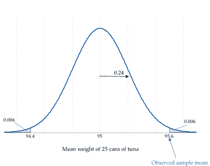
Figure 2: Distribution of the sample mean, \(\bar{X}\), based on a random sample of 25 tins of canned tuna from a Normally distributed population with mean 95 g and standard deviation 1.2 g.

The mean weight of 95.6 g is quite surprising, if the true mean weight of the cans is 95g. That is, a mean weight for 25 cans that is 0.6 g or more different from 95 g is a little unusual; the \(P\)-value quantifies this.

Next page - Theories about \(\mu\) - Connection between \(P\)-values and confidence intervals