Possible values of u

Possible values of $\mu$

In many research contexts, we may be curious to know about $\mu$, the population mean. In Inference for means, this was addressed by obtaining an interval which contains $\mu$ with a specified level of confidence.

Here we address our curiosity about $\mu$ in a different way. We ask: "Could $\mu$ be equal to a particular number?" "Are the data consistent with $\mu = 75$?"

You may wonder why this question is not posed much more directly. The question could be asked this way: "Is $\mu = 75$ ?" Why don't we just use this simple question? The answer is equally simple: since 75 is a very specific value, we know — without any collection of data — that this is almost certainly not the value of $\mu$. The value of $\mu$ in any example may be in an interval of the real line. Even if the true value of $\mu$ is in the vicinity of 75, it would be an utter fluke if it really was exactly that value. It might be 76.1, or 74.9, or 75.03, but it would be bizarre if it turned out to be exactly the queried value, that is, $\mu = 75.000...$.

On the other hand, the data may be consistent with a range of values for $\mu$, and it is possible that the data are consistent with $\mu = 75$, ...and also consistent with $\mu = 76.1$, and $\mu = 74.9$, and.... But, perhaps, not consistent with $\mu = 70$.

Interest in a particular value of $\mu$ in a population arises when there is a specification about the average value of a quantity. For regulatory purposes, for example, we might require that the stated quantity of a mass-produced food item, such as a can of tuna or a bar of chocolate, should be the average value of the population of such items. Another context is an engineering specification, for manufacturing purposes. We want the length of a component of a hydraulic pump to be 12 mm. We know that there will be variation among individual components, so they will not all be exactly 12 mm. But we do want them to be 12 mm on average; that is, we require $\mu = 12$.

It will usually be desirable also to think about the variation in the random variable, and require that to be small. Suppose that the chocolate bar is labelled as 100 g, and we get one which is 90 g. It would be small consolation to be told that the population average is 100 g, and receiving a bar of 90 g was just due to random variation: you were unlucky. Similarly, in the manufacturing context, small variation is important; specification limits define the acceptable range for the dimension of the component.

In statistical terms, this is saying that not only do we want to specify $\mu$, we want to ask for a small value of $\sigma$.

In this module, however, the focus is on the first of these: the value of the population mean $\mu$.

Cans of tuna

A particular brand of tuna has a stated amount of 95 g on the outside of the can. Suppose that the weight, $X$, of tuna in the can has a Normal distribution with mean $\mu = 95$ g and a standard deviation $\sigma = 1.2$ g. A random sample of 25 cans of this product is obtained, and the sample mean $\bar{x}$ is calculated. Are any of the following values for $\bar{x}$ surprising: $\bar{x} = 94.9,\bar{x} = 95.4,\bar{x} = 94.2?$

Solution

For the setting given, we know that the sample mean, $\bar{X}$, has a Normal distribution with mean 95 and variance $\tfrac{1.2^2}{25}$. That is, $\bar{X}\stackrel{\mathrm{d}}{\approx} \mbox{N}(95,\tfrac{1.2^2}{25})$. Note that this means the standard deviation of $\bar{X}$ is $\mbox{sd}(\bar{X}) = 1.2/5 = 0.24$. A plot of this distribution is shown below, with the positions of the three sample means indicated.

canned_tuna_dsn_of_sample_mean

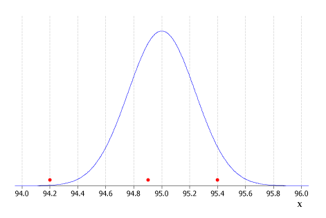
Figure 1: Distribution of the sample mean, $\bar{X}$, based on a random sample of weights of 25 cans of tuna from a Normally distributed population with mean 95g and standard deviation 1.2 g. Also shown are three possible sample means.

Among the three sample means contemplated:

$\bar{x} = 94.9$ is close to the expected value of the distribution (95 g) and hence is not surprising at all;
$\bar{x} = 95.4$ is towards the right hand tail of the distribution of $\bar{X}$ but is not large enough to be very surprising;
$\bar{x} = 94.2$ is a very unusual observation and surprisingly low.

How have we measured "surprising" in the canned tuna example? What makes us conclude that $\bar{x} = 94.2$ is a surprisingly low sample mean?

Note, firstly, that according to the given distribution of weights for the cans themselves, an individual can of weight 94.2 g would be not at all strange. The standard deviation, $\sigma$, for the weight distribution is 1.2 g, so a single can weight of 94.2 g is within one standard deviation of the mean (95 g).

But that is for a single can. It is a very different story when we consider the sample mean from a random sample of 25 cans. The distribution of $\bar{X}$, the sample mean, is much narrower; it has a standard deviation of 1.2/5 = 0.24. Hence an observation of 94.2 g for the sample mean is more than three standard deviations below the mean.

In this example, we have implicitly used the known distribution of the sample mean to produce a qualititative measure of surprise. We have looked at how far the sample mean is from the population mean, and taken into account the distribution of $\bar{X}$ in Figure 1.

Can we go further? It is useful to produce a quantitative measure of surprise. Since we know the distribution of $\bar{X}$, it can be used to obtain a formal probability that reflects our level of surprise in the observed sample mean, $\bar{x}$. This probability is based on the distribution of $\bar{X}$, and the observed sample mean, which we will denote by $\bar{x}_{\mbox{obs}}$. We determine

$$\Pr\left(|\bar{X} - \mu| \geq |\bar{x}_{\mbox{obs}} - \mu|\right).$$

In words: the probability that the distance between $\bar{X}$ and $\mu$ is at least as big as the distance between the observed sample mean and $\mu$.

Why "at least" as big? Suppose that on one day in a heat wave the maximum temperature is 44.3 degrees Celsius. This is very hot, and the media writes about it, because it is so extreme. There is interest in just how extreme such a day is, perhaps in terms of the historical record for our location. When this is done, we do not just ask how unusual are days with a maximum of exactly 44.3; we ask how rare are daily maximum temperatures of at least 44.3 degrees. In a conversation, someone mentions that "Jessica is really tall; there's only 1% of girls her age who are that tall". The same meaning applies: it is implied in this remark that 1% of girls who are Jessica's age are her height or taller.

In the same way, we always include more extreme values than that observed, in our assessment of how surprising or extreme we should regard a particular observed value of $\bar{x}$.

Exercise 2

For the canned tuna example, find the probability that the sample mean $\bar{X}$ is at least as far away from $\mu = 95$ as each of the three observed sample means considered:

$\bar{x} = 94.9$;
$\bar{x} = 95.4$;
$\bar{x} = 94.2.$

So far, we have assumed that the population distribution from which we are sampling is Normal, and that we know the population standard deviation $\sigma$. These are two features of the population or model, and in general we are making inferences about the population (notably, the population mean $\mu$). So it is reasonable to ask: can we avoid having to assume a Normal distribution and known $\sigma$?

As we saw in the module Inference for means, we can avoid making these assumptions, provided that we have a large enough sample size $n$. Due to the Central Limit Theorem, we can use, as an approximation for large $n$, the following result:

$$\frac{\bar{X} - \mu}{S/\sqrt{n}} \stackrel{\mathrm{d}}{\approx} \mbox{N}(0,1).\hspace{100pt}(1)$$

Cans of tuna (continued)

Suppose that we do not know that the distribution of weights of the individual cans is Normal, and we do not know the standard deviation, $\sigma$, of the distribution of weights. This is closer to what would happen in practice. We obtain a random sample of $n = 225$ cans. The average weight is found to be $\bar{x} = 94.8$ g and the standard deviation is $s = 1.4$ g, based on the sample. Is this an unusual sample, if the population mean is $\mu= 95$ g?

We obtain the result as follows. We require the probability that a sample mean from a sample of size $n= 225$ is at least as far from 95 g as the observed sample mean, $\bar{x} = 94.8 g$. The sample size is large, so we can use the result given in equation (1). We find that the required probability is

$$\Pr\left(\left|\frac{\bar{X} - 95}{S/\sqrt{225}}\right| \geq \left|\frac{94.8 - 95}{1.4/\sqrt{225}}\right| \right) \approx \Pr(|Z| \geq 2.1429) = 0.0321,$$

where $Z$ is the standard Normal distribution: $Z \stackrel{\mathrm{d}}{\approx} \mbox{N}(0,1)$. So for a random sample of $n =225$, when the standard deviation $s = 1.4$, a sample mean of 94.8 g is quite unusual.

In the canned tuna example, we have assumed that the population mean, $\mu = 95$ g, which is the quantity on the can's label. However, there are many situations where we would not want just to take the given population mean for granted. We might prefer to think of the population mean as unknown, which, in practice, it usually is. In that case, we regard assertions about the value of the population mean as hypotheses which may or may not be true.

Next page - Theories about $\mu$ - $P$-value

Possible values of \(\mu\)

Cans of tuna

Solution

Cans of tuna (continued)