Content

Standardising the sample mean

The module Exponential and normal distributions shows how any Normal distribution can be standardised, in the following way, to give a standard Normal distribution:

If \(Y \stackrel{\mathrm{d}}{=} \mathrm{N}(\mu,\sigma^2)\) and \(Z = \dfrac{Y-\mu}{\sigma}\), then \(Z \stackrel{\mathrm{d}}{=} \mathrm{N}(0,1)\).

The standard Normal distribution has mean 0 and variance 1. A random variable with this distribution is usually denoted by \(Z\). That is, \(Z \stackrel{\mathrm{d}}{=} \mathrm{N}(0,1)\).

Consider a standardisation of \(\bar{X}\). We subtract off the mean of \(\bar{X}\), which is \(\mu\), and divide through by the standard deviation of \(\bar{X}\), which is \(\dfrac{\sigma}{\sqrt{n}}\), to obtain a standardised version of the sample mean:

\[ \dfrac{\bar{X} - \mu}{\sigma/\sqrt{n}}. \]

Now we ask: What is the distribution of this quantity?

Sampling from a Normal distribution

We first consider the case of a random sample from a Normal population, say the population of study scores \(\mathrm{N}(30,7^2)\).

The standardisation of \(\bar{X}\) for this example is illustrated in figure 23. There are nine distributions in figure 23.

• The top row, moving from left to right, shows the distribution of the sample mean \(\bar{X}\) for random samples of size \(n = 30\), \(n = 50\) and \(n = 100\).
• The middle row shows the distributions of \(\bar{X} - \mu\); all the distributions are now centred at 0, but the spread of the distributions still varies, and still depends on \(n\).
• The bottom row shows the distributions of \(\dfrac{\bar{X} - \mu}{\sigma/\sqrt{n}}\); the three distributions of the standardised versions of \(\bar{X}\) have the same centre and spread. The mean is 0 and the standard deviation is 1.

Of course, all nine distributions in figure 23 are Normal distributions. As we saw in a previous section Sampling from symmetric distributions, if the parent distribution from which we are sampling is Normal, then the distribution of the sample mean is itself Normal, for any \(n\).

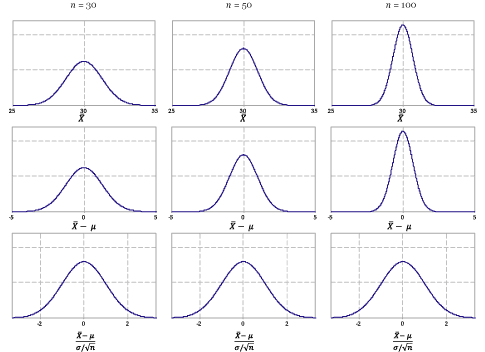
Figure 23: Standardisation of the distribution of \(\bar{X}\) for samples from a Normal distribution, for various values of \(n\).

In summary: For a random sample of size \(n\) from a Normal distribution,

\[ \dfrac{\bar{X} - \mu}{\sigma/\sqrt{n}} \stackrel{\mathrm{d}}{=} \mathrm{N}(0,1). \]

Under the specific conditions of sampling from a Normal distribution (and only then), this result holds for any value of \(n\).

Sampling from the uniform distribution

Now consider the distribution of the sample mean for random samples from the uniform distribution \(\mathrm{U}(0,1)\). We illustrate this in figure 24 with simulations of 100 000 samples.

• The top row, moving from left to right, shows the histogram of the sample mean \(\bar{X}\) for random samples of size \(n = 30\), \(n = 50\) and \(n = 100\). The histograms in the top row are symmetric and bell-shaped; there is greater variability when the means are based on smaller sample sizes.
• The middle row shows the histograms of \(\bar{X} - \mu\); all are now centred at 0, but the spread of the distributions still depends on \(n\), in the same way as it does in the top row.
• The bottom row shows the histograms of \(\dfrac{\bar{X} - \mu}{\sigma/\sqrt{n}}\). Now all of the histograms look very similar; they have the same centre and spread. The mean is 0 and the standard deviation is 1, and they are bell-shaped; in short, they have approximately the same distribution as \(Z \stackrel{\mathrm{d}}{=} \mathrm{N}(0,1)\).

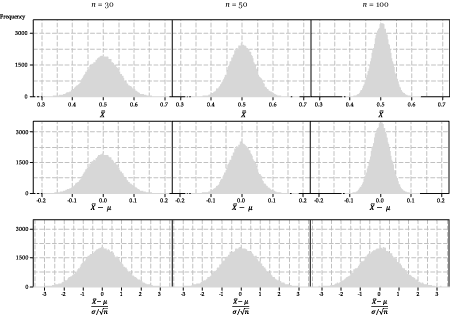
Figure 24: Standardisation of the distribution of \(\bar{X}\) for samples from a uniform distribution, for various values of \(n\).

This shows via simulation the application of the central limit theorem to the uniform distribution: for a random sample of size \(n\) from the uniform distribution, if \(n\) is large, then

\[ \dfrac{\bar{X} - \mu}{\sigma/\sqrt{n}} \stackrel{\mathrm{d}}{\approx} \mathrm{N}(0,1). \]

Sampling from the exponential distribution

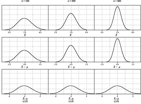
Next we consider standardisation of the distribution of sample means for samples from the exponential distribution with mean 7; see figure 25. This figure is based on the true distribution of the sample mean, as in this case it can be derived explicitly. (So we do not need to rely on histograms of sample means from many random samples to get an approximate idea of the distributions involved.)

Detailed description

Figure 25: Standardisation of the distribution of \(\bar{X}\) for samples from the exponential distribution \(\exp(\tfrac{1}{7})\), for various values of \(n\).

We have already seen the distribution of the sample mean \(\bar{X}\) based on random samples of size \(n=10\) from \(\exp(\dfrac{1}{7})\), in the section Sampling from asymmetric distributions (see figure 18). For the case \(n = 10\), the value of \(n\) is small and, although the distribution of \(\bar{X}\) is much more symmetric that the distribution of \(X\) itself, some skewness is still apparent.

Now, in figure 25, we look at considerably larger sample sizes.

• The top row of figure 25, moving from left to right, shows the distribution of the sample mean \(\bar{X}\) for random samples from \(\exp(\dfrac{1}{7})\) for \(n = 100\), \(n = 200\) and \(n = 400\).
• The middle row shows the distributions of \(\bar{X} - \mu\); all the distributions are centred at 0, but the spread of the distributions still depends on \(n\).
• The bottom row shows the distributions of \(\dfrac{\bar{X} - \mu}{\sigma/\sqrt{n}}\); now all the distributions have the same centre and spread. The mean is 0 and the standard deviation is 1.

For these larger values of \(n\), can you still detect some skewness visually? Are these distributions symmetric? There is some slight skewness apparent… but you have to look hard! The distribution is approximately Normal, and the approximation is quite good for these large values of \(n\).

Keep in mind how good this approximation is for these values of \(n\), given the substantial skewness of the parent exponential distribution.

This shows the application of the central limit theorem to the exponential distribution: for a random sample of size \(n\) from the exponential distribution, if \(n\) is large, then

\[ \dfrac{\bar{X} - \mu}{\sigma/\sqrt{n}} \stackrel{\mathrm{d}}{\approx} \mathrm{N}(0,1). \]

We have shown examples for the uniform and exponential distributions, but the conditions of the central limit theorem are completely general: it works for any distribution with a finite mean \(\mu\) and finite variance \(\sigma^2\).

The Normal approximation described here is used later, when we obtain an approximate confidence interval for the unknown population mean \(\mu\), based on a random sample. Before getting to the practicalities, however, we consider some very important general ideas about confidence intervals.

Next page - Content - Population parameters and sample estimates