Content

Sampling from symmetric distributions

We found the mean and variance of the sample mean \(\bar{X}\) in the previous section. What more can be said about the distribution of \(\bar{X}\)? We now consider the shape of the distribution of the sample mean.

It is instructive to consider random samples from a variety of parent distributions.

Sampling from the Normal distribution

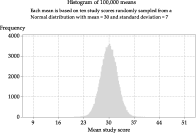
When exploring the concept of a sample mean as a random variable, we used the example of sampling from a Normal random variable. Specifically, we considered taking a random sample of size \(n=10\) from the \(\mathrm{N}(30,7^2)\) distribution. figure 5 illustrated an approximation to the distribution of \(\bar{X}\) in this case, by showing a histogram of 100 sample means from random samples of size \(n=10\).

To approximate the distribution better, we take a lot more samples than 100. figure 6 shows a histogram of 100 000 sample means based on 100 000 random samples each of size \(n=10\). Each of the random samples is taken from the Normal distribution \(\mathrm{N}(30,7^2)\).

Detailed description

Figure 6: Histogram of means from 100 000 random samples of size \(n=10\) from \(\mathrm{N}(30,7^2)\).

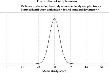
Although 100 000 is a lot of samples, it is still not quite an 'endless' repetition! If we took more and more samples of size 10, each time obtaining the sample mean and adding it to the histogram, then the shape of the histogram would become smoother and smoother and more and more bell-shaped, until eventually it would become indistinguishable from the shape of the Normal curve shown in figure 7.

figure 7 shows the true distribution of sample means for samples of size \(n=10\) from \(\mathrm{N}(30,7^2)\), which is only approximated in figures 5 and 6.

Detailed description

Figure 7: The distribution of the sample mean \(\bar{X}\) based on random samples of size \(n=10\) from \(\mathrm{N}(30,7^2)\), with \(\bar{X} \stackrel{\mathrm{d}}{=} \mathrm{N}(30,\dfrac{7^2}{10})\).

If we are sampling from a Normal distribution, then the distribution of \(\bar{X}\) is also Normal, a result which we assert without proof. This result is true for all values of \(n\).

Theorem (Sampling from a Normal distribution)

If we have a random sample of size \(n\) from the Normal distribution with mean \(\mu\) and variance \(\sigma^2\), then the distribution of the sample mean \(\bar{X}\) is Normal, with mean \(\mu\) and variance \(\dfrac{\sigma^2}{n}\). In other words, for a random sample of size \(n\) on \(X \stackrel{\mathrm{d}}{=} \mathrm{N}(\mu,\sigma^2)\), the distribution of the sample mean is itself Normal: specifically, \(\bar{X} \stackrel{\mathrm{d}}{=} \mathrm{N}(\mu,\tfrac{\sigma^2}{n})\).

We have observed that the spread of the distribution of \(\bar{X}\) is less than that of the distribution of the parent variable \(X\). This reflects the intuitive idea that we get more precise estimates from averages than from a single observation. Further, since the sample size \(n\) is in the denominator of the variance of \(\bar{X}\), the spread of sample means in a long-run sequence based on samples of size \(n=1000\) each time (for example) will be smaller than the spread of sample means in a long-run sequence based on samples of size \(n=50\).

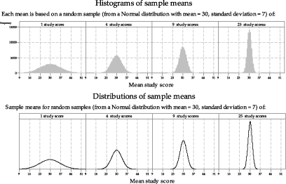
Again consider taking repeated samples of study scores from the Normal distribution \(\mathrm{N}(30,7^2)\). Four different scenarios are shown in figure 8, each based on different sample sizes of study scores: \(n = 1\), \(n = 4\), \(n = 9\) and \(n = 25\). In the top panel are histograms based on 100 000 sample means, and in the bottom panel are the true distributions of the sample means. The distributions of sample means based on larger sample sizes are narrower, and more concentrated around the mean \(\mu\), than those based on smaller samples. The distribution of sample means based on one study score is, of course, identical to the original population distribution of study scores.

Detailed description

Figure 8: Histograms and true distributions of means of random samples of varying size from \(\mathrm{N}(30,7^2)\).

In summary: For a random sample of size \(n\) on \(X \stackrel{\mathrm{d}}{=} \mathrm{N}(\mu,\sigma^2)\), the distribution of \(\bar{X}\) is itself Normal; specifically,

\[ \bar{X} \stackrel{\mathrm{d}}{=} \mathrm{N}(\mu,\tfrac{\sigma^2}{n}). \]

It is very important to understand that sampling from a Normal distribution is a special case. It is not true, for other parent distributions, that the distribution of \(\bar{X}\) is Normal for any value of \(n\).

We now consider the distribution of sample means based on populations that do not have Normal distributions.

Sampling from the uniform distribution

Recall that the uniform distribution is one of the continuous distributions, with the corresponding random variable equally likely to take any value within the possible interval. If \(X \stackrel{\mathrm{d}}{=} \mathrm{U}(0,1)\), then \(X\) is equally likely to take any value between 0 and 1.

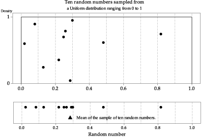
figure 9 shows the first of several random samples of size \(n=10\) from the uniform distribution \(\mathrm{U}(0,1)\), as seen in the module Random sampling . The sample has been projected down to the \(x\)-axis in the lower part of figure 9 to give a dotplot of the data, and now the sample mean is added as a black triangle under the dots. The data in this case are referred to as 'random numbers', since a common application of the \(\mathrm{U}(0,1)\) distribution is to generate random numbers between 0 and 1.

figure 10 shows ten samples, each of 10 observations from the same uniform distribution \(\mathrm{U}(0,1)\). The top panel shows the population distribution. The middle panel shows each of the ten samples, with dots for the observations and a triangle for the sample mean. The bottom panel shows the ten sample means plotted on a dotplot.

Detailed description

Figure 9: First random sample of size \(n=10\) from \(\mathrm{U}(0,1)\), with the sample mean shown as a triangle.

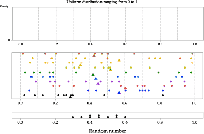
Detailed description

Figure 10: Ten random samples of size \(n=10\) from \(\mathrm{U}(0,1)\), with the sample means shown as triangles in the middle panel and as dots in the dotplot in the bottom panel.

figure 11 shows a histogram with one million sample means from the same population distribution. There are several features to note in figure 11. As in the case of the distribution of sample means taken from a Normal population, the spread in the histogram of sample means is less than the spread in the parent distribution from which the samples are taken. However, in contrast to the case of sampling from a Normal distribution, the shape of the histogram is unlike the population distribution; rather, it is like a Normal distribution.

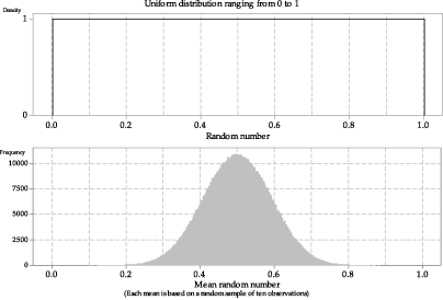
Detailed description

Figure 11: Histogram of means from one million random samples of size \(n=10\) from \(\mathrm{U}(0,1)\).

figure 12 shows four different histograms of means of samples of random numbers taken from the uniform distribution \(\mathrm{U}(0,1)\). From left to right, they are based on sample size \(n = 1\), \(n = 4\), \(n = 16\) and \(n = 25\). Of course, when the sample mean is based on a single random number (\(n = 1\)), the shape of the histogram looks like the original parent distribution. The other histograms are not uniform; they tend to be bell-shaped. It is rather remarkable that we see this is so even for a sample size as small as \(n=4\).

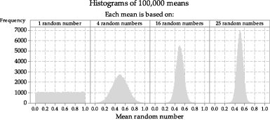
Figure 12: Histograms of means of random samples of varying size from \(\mathrm{U}(0,1)\).

How does this tendency to a bell-shaped curve arise?

Consider the means of samples of size \(n=4\), for example. figure 13 shows ten different random samples taken from the uniform distribution \(\mathrm{U}(0,1)\), each with four observations. The observations are shown as dots, and the means of the samples of four observations are shown as triangles. The darker vertical line at \(x = 0.5\) shows the true mean for the population from which the samples were taken.

Consider the values of the observations sampled in relation to the population mean. The first sample in figure 13 has two values below \(0.5\), and two above; the mean of these four values is close to 0.5. The second sample is similar, with two values below the true mean, and two values above. Samples 3, 6 and 7 have three values below the mean, and only one above. The means of these three samples are below the true mean, and they tend to be further from 0.5 than samples 1 and 2. All four observations in sample 8 are above \(0.5\), and all four observations in sample 10 are below \(0.5\); the means of these two samples are farthest from the true population mean.

As the population from which the observations are sampled is uniform, samples with two of the four observations above the mean of 0.5 will arise more often than samples with one or three observations above \(0.5\); samples with zero or four observations above 0.5 will arise least often. Hence, we see the tendency for the histogram in the second panel in figure 12 to be concentrated and centred around 0.5.

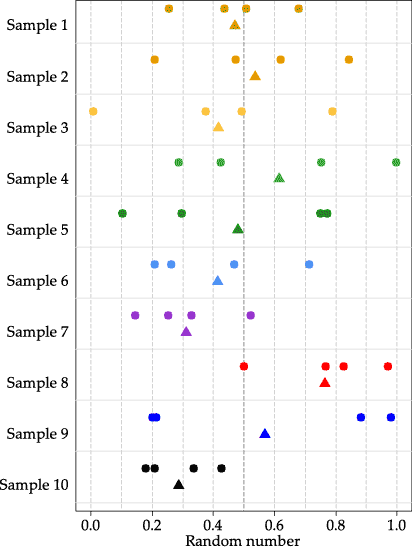
Figure 13: Ten random samples of size \(n=4\) from \(\mathrm{U}(0,1)\), with the sample means shown as triangles.

Next page - Content - Sampling from asymmetric distributions