Content

The sample mean as a random variable

In the module Random sampling , we examined the variability of samples of a fixed size \(n\) from a variety of continuous population distributions. We saw, for example, a number of random samples of size \(n = 10\) from a Normal population with mean \(\mu = 30\) and standard deviation \(\sigma = 7\). The population modelled by this distribution is the population of study scores of Year 12 students in a given subject.

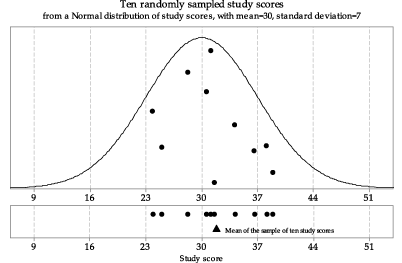
figure 1 is the first set of ten randomly sampled study scores from \(\mathrm{N}(30,7^2)\) shown in the module Random sampling . The sample has been projected down to the \(x\)-axis in the lower part of figure 1 to give a dotplot of the data, and now the sample mean is shown as a black triangle under the dots.

Detailed description

Figure 1: First random sample of size \(n=10\) from \(\mathrm{N}(30,7^2)\), with the sample mean shown as a triangle.

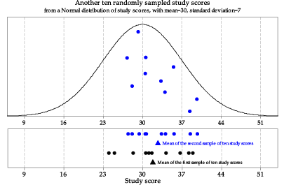
figure 2 shows another random sample of size 10 from the same parent Normal distribution \(\mathrm{N}(30,7^2)\). The lower part of figure 2 shows both the first and second samples and their means. We see that repeated samples from the same distribution have different means — this is something we would expect, given that the observations in the repeated samples from the same distribution are different from each other. It is the variation in sample means that we focus on in this module.

Detailed description

Figure 2: Second random sample of size \(n=10\) from \(\mathrm{N}(30,7^2)\).

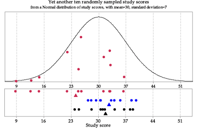
figure 3 shows the third sample from the same underlying Normal distribution \(\mathrm{N}(30,7^2)\).

Detailed description

Figure 3: Third random sample of size \(n=10\) from \(\mathrm{N}(30,7^2)\).

Now we consider the three samples we have already from \(\mathrm{N}(30,7^2)\), and another seven samples of size \(n = 10\) from this distribution. The middle panel of figure 4 shows the means of these ten samples, but not the individual study scores sampled. The bottom panel of figure 4 shows the same ten sample means as a dotplot. This describes the distribution of the ten mean study scores from ten different random samples from \(\mathrm{N}(30,7^2)\).

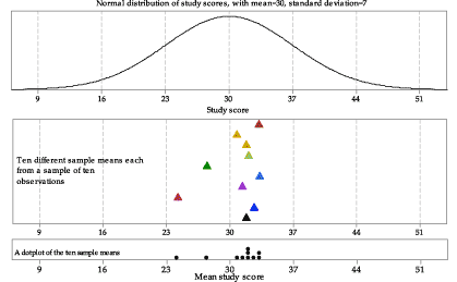
Figure 4: Means from ten random samples of size \(n=10\) from \(\mathrm{N}(30,7^2)\).

We extend this idea in figure 5, which shows a histogram of the means of 100 samples of size 10 from the Normal distribution \(\mathrm{N}(30,7^2)\). The choice of 100 as the number to show is arbitrary; all that is intended is to show a large enough number of sample means to provide an idea of how much variation there can be among such sample means. figure 5 shows the population distribution from which the samples are taken in the top panel, and the histogram of sample means in the bottom panel.

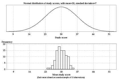
Detailed description

Figure 5: Histogram of means from 100 random samples of size \(n=10\) from \(\mathrm{N}(30,7^2)\).

There are a number of features to note in figure 5. The sample means are roughly centred around 30. They range in value from about 24 to 35. There is variability in the sample means, but it is smaller than the variability in the population from which the samples were taken. The third sample mean, shown in red in figure 3, appears to be quite different from the first and second sample means; it is represented in the lowest bar of the histogram in figure 5.

In summary: The sample mean \(\bar{X}\) is a random variable, with its own distribution.

Next page - Content - The mean and variance of \(\bar{X}\)