Content
Calculating confidence intervals
Calculating a 95% confidence interval with the Normal approximation
We have seen that the sample mean \(\bar{X}\) has mean \(\mu\) and variance \(\dfrac{\sigma^2}{n}\), and that the distribution of \(\bar{X}\) is approximately Normal when the sample size \(n\) is large. This raises the question: How large is 'a large sample size'? Appropriate guidelines need to take into account the nature of the population being sampled, as far as this is possible; this will be elaborated later in this section.
The Normal approximation for the distribution of \(\bar{X}\) tells us that, for large \(n\),
\[ \dfrac{\bar{X} - \mu}{\sigma/\sqrt{n}} \stackrel{\mathrm{d}}{\approx} \mathrm{N}(0,1). \]For a random variable with the standard Normal distribution, \(Z \stackrel{\mathrm{d}}{=} \mathrm{N}(0,1)\), we know that \(\Pr(-2 < Z < 2) \approx 0.95\). To be more precise:
\[ \Pr(-1.96 < Z < 1.96) = 0.95. \]We studied how to obtain the value 1.96 in the module Exponential and normal distributions . figure 29 is a visual reminder.
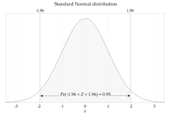
Figure 29: The standard Normal distribution, \(Z \stackrel{\mathrm{d}}{=} \mathrm{N}(0,1)\).
If we consider the Normal approximation to the distribution of the standardised sample mean, it follows that we can state that, for large \(n\),
\[ \Pr\Bigl(-1.96 < \dfrac{\bar{X} - \mu}{\sigma/\sqrt{n}} < 1.96 \Bigr) \approx 0.95. \]We multiply through by \(\dfrac{\sigma}{\sqrt{n}}\) to obtain
\[ \Pr\Bigl(-1.96 \dfrac{\sigma}{\sqrt{n}} < \bar{X} - \mu < 1.96 \dfrac{\sigma}{\sqrt{n}}\Bigr) \approx 0.95. \]In other words, the distance between \(\bar{X}\) and \(\mu\) will be less than \(1.96 \dfrac{\sigma}{\sqrt{n}}\) for 95% of sample means.
One further rearrangement gives
\[ \Pr\Bigl(\bar{X} - 1.96 \dfrac{\sigma}{\sqrt{n}} < \mu < \bar{X} + 1.96 \dfrac{\sigma}{\sqrt{n}}\Bigr) \approx 0.95. \]It is really important to reflect on this probability statement. Note that it has \(\mu\) in the centre of the inequalities. The population parameter \(\mu\) does not vary: it is fixed, but unknown. The random element in this probability statement is the random interval around \(\mu\).
This forms the basis for the approximate 95% confidence interval for the true mean \(\mu\). In a given case, we have just a single sample mean \(\bar{x}\). An approximate 95% confidence interval for \(\mu\) is given by
\[ \bar{x} \pm 1.96 \dfrac{\sigma}{\sqrt{n}}. \]However, a problem remains. The uncertainty in the estimate depends on \(\sigma\), which is an unknown parameter: the true standard deviation of the parent distribution.
In the approximate methods used here, we replace the population standard deviation \(\sigma\) with the sample standard deviation.
The sample standard deviation is an estimate of the population standard deviation. Just as \(\bar{X}\) is a random variable that estimates \(\mu\) and has an observed value \(\bar{x}\) for a specific sample, so \(S\) is a random variable that estimates \(\sigma\) and has an observed value \(s\) for a specific sample. The sample standard deviation (which is dealt with in the national curriculum in Year 10) is defined as follows. For a random sample \(X_1, X_2, \dots, X_n\) from a population with standard deviation \(\sigma\), the sample standard deviation is defined to be
\[ S = \sqrt{\dfrac{\sum_{i=1}^n (X_i - \bar{X})^2}{n-1}}, \]where \(\bar{X}\) is the sample mean. For a specific random sample \(x_1, x_2, \dots, x_n\), the observed value of the sample standard deviation is
\[ s = \sqrt{\dfrac{\sum_{i=1}^n (x_i - \bar{x})^2}{n-1}}, \]where \(\bar{x}\) is the observed value of the sample mean.
It is reasonable to ask whether using \(S\) in place of \(\sigma\) actually works. We have extensively demonstrated the approximate Normality of the distribution of the sample mean. In particular, we have seen that, for large \(n\),
\[ \dfrac{\bar{X} - \mu}{\sigma/\sqrt{n}} \stackrel{\mathrm{d}}{\approx} \mathrm{N}(0,1). \]But now it seems that we are going to rely on a different, further approximation, that for large \(n\),
\[ \dfrac{\bar{X} - \mu}{S/\sqrt{n}} \stackrel{\mathrm{d}}{\approx} \mathrm{N}(0,1). \]The result that uses \(S\) in place of \(\sigma\) is also valid; as \(n\) tends to infinity, the sample standard deviation \(S\) gets closer and closer to the true standard deviation \(\sigma\). We could revisit all of the previous examples and demonstrate this for the uniform, exponential and so on; instead, we use the strange-looking distribution to make the point.
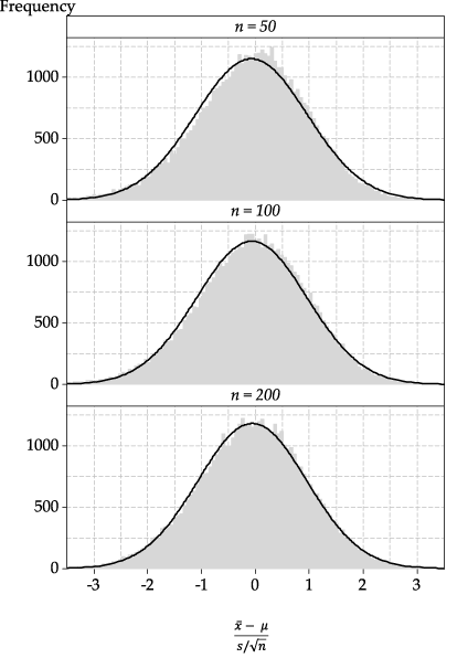
figure 30 shows histograms of \(\dfrac{\bar{X} - \mu}{S/\sqrt{n}}\), for various values of \(n\), based on random samples from the strange distribution considered in the section Sampling from asymmetric distributions (see figure 22). Superimposed Normal distributions are added to enable a visual assessment of the adequacy of the Normal approximation.
Detailed description
Figure 30: Histograms of the standardised sample mean, using the sample standard deviation in the denominator, rather than the population standard deviation, for various values of \(n\).
The standardised distributions in figure 30 using \(S\) in the denominator do not approximate Normality as well as the histograms of \(\bar{X}\) in figure 22; some skewness is evident. But for \(n=200\), the approximation is good; keep in mind that we are sampling from a decidedly odd parent distribution here.
Hence, for large \(n\), based on a random sample from a distribution with mean \(\mu\) and standard deviation \(\sigma\), an approximate 95% confidence interval for \(\mu\) is given by
\[ \bar{x} \pm 1.96 \dfrac{s}{\sqrt{n}}. \]Example: Internet use by children
A recent large survey of a random sample of Australian children asked about weekly hours of internet use in three age groups. The following table shows the mean and standard deviation of the number of hours of internet use per week and the total number of children surveyed for each age group.
| Age group (years) | Mean (hours/week) | Standard deviation | Number surveyed |
| 5–8 | 3.29 | 4.29 | 2150 |
| 9–11 | 5.75 | 6.17 | 2530 |
| 12–14 | 9.95 | 7.81 | 1250 |
Calculate an approximate 95% confidence interval for the mean number of hours of internet use per week in each group.
Solution
For the 5–8 age group, we have \(\bar{x} = 3.29\) and
\[ 1.96 \dfrac{s}{\sqrt{n}} = 1.96 \dfrac{4.29}{\sqrt{2150}} = 0.181. \]Hence, the 95% confidence interval is \(3.29 \pm 0.181\), or \((3.11, 3.47)\), hours per week.
For the 9–11 age group, we have \(\bar{x} = 5.75\) and
\[ 1.96 \dfrac{s}{\sqrt{n}} = 1.96 \dfrac{6.17}{\sqrt{2530}} = 0.240. \]Hence, the 95% confidence interval is \(5.75 \pm 0.240\), or \((5.51, 5.99)\), hours per week.
For the 12–14 age group, we have \(\bar{x} = 9.95\) and
\[ 1.96 \dfrac{s}{\sqrt{n}} = 1.96 \dfrac{7.81}{\sqrt{1250}} = 0.433. \]Hence, the 95% confidence interval is \(9.95 \pm 0.433\), or \((9.52, 10.38)\), hours per week.
Exercise 5
Consider the approximate 95% confidence interval calculated in the previous example for the 12–14 age group. Decide if each of the following statements is true or false. In each case, explain why.
- It is plausible that Australian children aged 12–14 use the internet for an average of 10 hours per week.
- Most children in this age group use the internet for between 9.52 and 10.38 hours per week.
- No child in this age group could use the internet for 24 hours per week.
Exercise 6
Casey buys a Venus chocolate bar every day. The wrapper on the Venus bar claims the weight is 53 grams. Casey decides to investigate this claim by weighing each Venus bar he purchases, every day, for six weeks. He uses a scale that is accurate to 0.1 grams. The following figure shows a dotplot of the 42 weights.
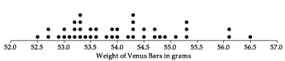
Figure 31: Dotplot of the weights of 42 Venus bars.
Casey decides to regard the claim on the wrapper as a claim about \(\mu\), the true average weight of all Venus bars manufactured. The sample mean of the 42 weights is 54.0 grams, and the sample standard deviation is 0.98 grams.
- Consider the claim on the Venus bar wrapper. Do you think that the claim is plausible, considering the sample mean of the 42 Venus bars?
- Find an approximate 95% confidence interval for the true mean weight of Venus bars, based on Casey's sample.
- Again consider the claim on the Venus bar wrapper. Is the claim plausible, considering the confidence interval?
- What assumptions have been made about Casey's sample of Venus bars?
Calculating a \(C\%\) confidence interval with the Normal approximation
We have focussed so far on 95% confidence intervals, since 95% is the confidence level that is used most commonly. The general form of an approximate \(C\%\) confidence interval for a population mean is
\[ \bar{x} \pm z \dfrac{s}{\sqrt{n}}, \]where the value of \(z\) is appropriate for the confidence level. For a 95% confidence interval, we use \(z=1.96\), while for a 90% confidence interval, for example, we use \(z=1.64\).
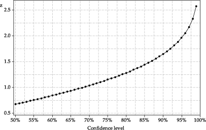
In general, for a \(C\%\) confidence interval, we need to find the value of \(z\) that satisfies
\[ \Pr(-z < Z < z) = \dfrac{C}{100}, \quad\text{whe re } Z \stackrel{\mathrm{d}}{=} \mathrm{N}(0,1). \]figure 32 shows the required value of \(z\) as a function of the confidence level.
Detailed description
Figure 32: The relationship between the confidence level and the value of \(z\) in the formula for an approximate confidence interval.
The following figure is a repeat of figure 28. It shows confidence intervals based on the same estimated mean, but with different confidence levels. The larger confidence levels lead to wider confidence intervals.
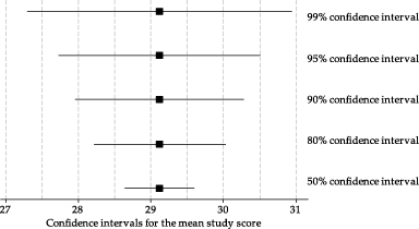
Figure 33: Confidence intervals from the same data, but with different confidence levels.
The distance from the sample estimate \(\bar{x}\) to the endpoints of the confidence interval is
\[ E = z \dfrac{s}{\sqrt{n}}. \]The quantity \(E\) is referred to as the margin of error. The margin of error is half the width of the confidence interval. Sometimes confidence intervals are reported as \(\bar{x} \pm E\); for example, as \(9.95 \pm 0.43\). This means that the lower and upper bounds of the interval are not directly stated, but must be derived.
In figure 33, we see larger margins of error when the confidence level is larger. This is because the value of \(z\) from the standard Normal distribution will be larger when the confidence level is larger.
We use a confidence interval when we want to make an inference about a population parameter, in this case, the population mean. The confidence interval describes a range of plausible values for the population mean that could have given rise to our random sample of observations. The margin of error in a confidence interval for the mean is based on the standard deviation divided by the square root of sample size; generally, the margin of error for a confidence interval will be smaller than the standard deviation of the sample, unless the sample size is very small.
Sometimes a confidence interval is wrongly interpreted as providing information about plausible values for the range of the data. This is illustrated in the next example.
Example: Venus bar weights
The following figure shows the 42 Venus bar weights considered in exercise 6, and shows a 95% confidence interval for the true mean weight. The confidence interval is relatively narrow, describing plausible values for the population mean that could have given rise to the sample of 42 weights.
The figure also shows the sample mean \(\pm 1.96\) times the sample standard deviation. The range \(\bar{x} \pm 1.96s\) is an interval that estimates the central 95% of the distribution of \(X\), based on the estimates of the mean and standard deviation, assuming the random sample comes from a Normal distribution.
As the figure shows, it is completely wrong to say that 'about 95% of the distribution of \(X\) is estimated to be between the ends of the 95% confidence interval'.
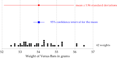
Figure 34: Comparison of a confidence interval for \(\mu\) and an interval estimated to include the central 95% of the distribution of \(X\).
Example: Internet use by children
Continuing with the internet-use example, consider the 12–14 age group. Calculate an approximate 90% confidence interval for the true mean number of hours of internet use per week in this group.
Solution
As before, we have \(\bar{x} = 9.95\). The margin of error is
\[ 1.64 \dfrac{s}{\sqrt{n}} = 1.64 \dfrac{7.81}{\sqrt{1250}} = 0.362. \]Hence, the 90% confidence interval is \(9.95 \pm 0.362\), or \((9.59, 10.31)\).
Exercise 7
Consider Casey's sample of Venus bars from exercise 6. Rather than a 95% confidence interval for the true mean weight of Venus bars, consider an approximate 80% confidence interval.
- Without calculating the 80% confidence interval, guess the lower and upper bounds.
- Find the appropriate factor \(z\) from the standard Normal distribution for an 80% confidence interval (if necessary, by reading it off the graph in figure 32). Consider the ratio of the values of \(z\) for the 80% and 95% confidence intervals, and estimate the lower and upper bounds of the 80% confidence interval.
- Calculate the approximate 80% confidence interval for the true mean weight, based on Casey's sample of Venus bars.
- Consider the claim on the wrapper about the weight. Comment on this, based on the 80% confidence interval.
Exercise 8
A recent large survey of Australian households estimated the average weekly household expenditure on clothing and footwear to be $44.50, with a standard deviation of $145.80. The margin of error was reported to be $2.90, for a 95% confidence interval.
- What shape is the distribution of weekly household expenditure on clothing and footwear likely to be?
- Is the shape of the distribution of weekly household expenditure on clothing and footwear a concern, if you wish to estimate the true mean of weekly household expenditure on clothing and footwear?
- Based on the information provided, approximately how many households were surveyed?
- Find a 95% confidence interval for the true mean weekly household expenditure on clothing and footwear.
- Use the results of this survey to estimate the mean yearly household expenditure on clothing and footwear. What is the 95% confidence interval?
When to use the Normal approximation
We have seen in this module that, for large \(n\), an approximate 95% confidence interval for \(\mu\) is
\[ \bar{x} \pm 1.96 \dfrac{s}{\sqrt{n}}. \]It is pertinent to ask: How large is 'large'? In effect, what is the smallest sample size for which the approximation is adequate?
A commonly cited guideline is that \(n\) should be greater than 30. However this guideline does not apply in all cases; sometimes larger sample sizes are needed to safely assume that the Normal approximation is appropriate. Here are some more detailed guidelines:
- If the population sampled has a Normal distribution, then \(\dfrac{\bar{X} - \mu}{S/\sqrt{n}} \stackrel{\mathrm{d}}{\approx} \mathrm{N}(0,1)\), provided the sample size is greater than 30.
- If the population sampled has a symmetric distribution, then \(\dfrac{\bar{X} - \mu}{S/\sqrt{n}} \stackrel{\mathrm{d}}{\approx} \mathrm{N}(0,1)\), provided the sample size is greater than 30.
- If the population sampled has a somewhat skewed distribution, then \(\dfrac{\bar{X} - \mu}{S/\sqrt{n}} \stackrel{\mathrm{d}}{\approx} \mathrm{N}(0,1)\), provided the sample size is greater than 60. Here, 'somewhat skewed' means that the distribution is not symmetric but is not as skewed as an exponential distribution.
- If the population sampled has an exponential distribution, then \(\dfrac{\bar{X} - \mu}{S/\sqrt{n}} \stackrel{\mathrm{d}}{\approx} \mathrm{N}(0,1)\), provided the sample size is greater than 130.
These guidelines are summarised in the following table.
| Parent distribution | Required sample size \(n\) |
|---|---|
| Normal | \(n > 30\) |
| Symmetric | \(n > 30\) |
| Somewhat skewed | \(n > 60\) |
| Exponential | \(n > 130\) |
figure 35 provides four example populations. In the top row, from left to right, there is a Normal population, an example of a symmetric distribution (in this case, a triangular distribution), a somewhat skewed distribution and an exponential distribution. In the bottom row, under each distribution, is a random sample. The size of the samples shown correspond to the guidelines in the table. Samples of size \(n = 30\) are taken from the Normal and symmetric populations, a sample of size \(n = 60\) is taken from the skewed distribution, and a sample of size \(n = 130\) from the exponential distribution. The samples from the skewed and exponential distributions appear to be more clearly skewed than those from the Normal and triangular distributions.
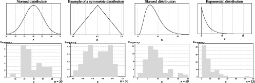
Figure 35: Examples of samples from four different populations.
In practice, when calculating a confidence interval for a population mean based on a random sample, we may not have information about the population from which the sample was taken. But we do have the random sample itself! We need to make a judgement about the likely population distribution from which the sample arose. figure 36 gives examples of ten different samples from each of the four different populations shown in the top part of figure 35. It is possible to get some idea of the shape of the parent distribution from the histogram of the random sample itself, and that may assist us to judge whether the sample size is large enough for the Normal approximation to be adequate.
An important overall message, however, is that sample sizes of a few hundred or so are enough for the use of the Normal approximation in general, unless the parent distribution is really bizarre.
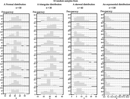
Figure 36: Ten samples from each of four different populations.
Next page - Answers to exercise
| This publication is funded by the Australian Government Department of Education, Employment and Workplace Relations |
Contributors Term of use |