Content

Confidence intervals

This section deals with fundamental aspects of confidence intervals. In the next section, we will deal with obtaining a confidence interval for the specific case we are considering, but it is important first to understand confidence intervals conceptually.

A sample mean \(\bar{x}\) is a single point or value that provides us with an estimate of the true mean of interest in the population. In some sense, we are not interested in the particular value of the sample mean per se, but rather we are interested in the information it provides us about the population. It provides an estimate of the population parameter of interest; in this case, the mean in the population, \(\mu\).

While the mean from the sample will provide us with the best estimate of the population mean, it is unlikely that the sample value will be exactly equal to the parameter being estimated. Hence, the sample estimate is most useful if it is combined with some information about its precision.

Suppose, for example, we want to estimate the mean \(\mu\) of study scores for a particular Year 12 subject, and that we have two different random samples of study scores for this subject available. The first sample provides an estimate of the true mean of \(29.1\), while the second sample provides the estimate 27.5. These estimates may seem inconsistent, and it may be unclear which we might prefer to rely on. However, if the first sample mean is likely to be within \(\pm 1.4\) of the true value of \(\mu\), and the second sample mean is likely to be within \(\pm 5.0\) of the true value of \(\mu\), then the first result is more precise than the second.

By describing the first result as \(29.1 \pm 1.4\), we are specifying an interval or range of values (from \(29.1 - 1.4\) to \(29.1 + 1.4\)) within which we have confidence that the true value of \(\mu\) lies. The interval has a lower bound and an upper bound: 27.7 and \(30.5\), respectively. This interval is an indicator of the precision of the estimate of the population mean and is called a confidence interval. 'Confidence' has a particular meaning in this context, which we now describe.

Confidence level

In working out a confidence interval, we decide on a 'degree' or 'level' of confidence. This is quantified by the confidence level. In most applications, the confidence level used is 95%.

The confidence level specifies the long-run percentage or proportion of confidence intervals containing the true value — in this context, \(\mu\). Illustrating this idea requires a simulation or a thought experiment. In practice, we typically have a single sample of \(n\) observations, and we calculate \(\bar{x}\) and a single confidence interval to characterise the precision in the result. Any actual interval either contains or does not contain the true value of the parameter \(\mu\). We don't know, for example, if the interval 27.7 to 30.5 for the mean study score contains the true value. The confidence level — 95% in this example — does not mean that the chance of this particular interval containing \(\mu\) is 0.95.

To illustrate the meaning of the confidence level, assume we know that the value of the true mean study score \(\mu\) is 30. The first random sample described above was based on 100 students and the mean was 29.1. We can imagine repeating this process many times, sampling different students each time, and each time we will observe a different sample mean.

figure 26 shows the estimates and 95% confidence intervals from 100 such random samples, with the first result closest to the \(x\)-axis. For each random sample, the estimate of the mean of interest is plotted as a dot in the centre of a line. The line shows the 95% confidence interval for the particular random sample. For the first random sample, the line showing the 95% confidence interval is from 27.7 to 30.5.

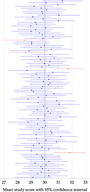
Figure 26: 95% confidence intervals for the mean study score from 100 random samples, each of 100 students.

The darker vertical line in figure 26 corresponds to the true value of \(\mu = 30\). Most of the confidence intervals are colored blue, but a small number are red; these are the confidence intervals that do not include the true value of 30. In total, four of the 100 intervals are red. In this small simulation, 96% of the intervals include the true value. We expect that, on average, 95% of the 95% confidence intervals will include the true value, and this is the real meaning of the '95%'; with much larger simulations, the percentage would be very close to 95%.

Varying the confidence level

figure 27 shows the same 100 random samples of 100 students again. For each random sample, the estimate of the mean of interest is plotted as a dot in the centre of a line which this time shows the 50% confidence interval. Because they represent the same samples, the dots in figure 27 are at the same positions as those in figure 26.

Red lines correspond to confidence intervals that do not include the true value of the parameter \(\mu = 30\). The 50% confidence intervals look narrow and precise, but figure 27 indicates that this is at a price. The intervals are narrower than the 95% confidence intervals in figure 26, but around half of them do not include the true value of the parameter.

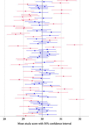
Figure 27: 50% confidence intervals for the mean study score from 100 random samples, each of 100 students.

Consider figure 28, which shows confidence intervals for the mean study score from the first random sample described above. The confidence intervals have different confidence levels. When the confidence level is larger, the confidence interval is wider. This is a natural consequence of the higher probability of including the true parameter value, in the imagined long-run sequence of repetitions.

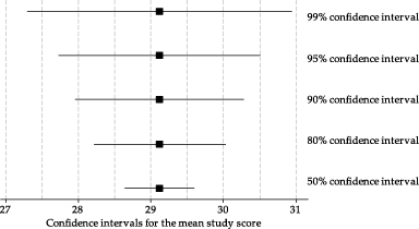
Figure 28: Estimate of the mean study score from one random sample, with confidence intervals using different confidence levels.

Next page - Content - Calculating confidence intervals