Content
More on calculating confidence intervals
Calculating a C% confidence interval with the Normal approximation
We have focussed so far on 95% confidence intervals, which is the confidence level that is used most commonly. The general form of an approximate \(C\%\) confidence interval for a population proportion is
\[ \hat{p} \pm z \sqrt{\dfrac{\hat{p}(1-\hat{p})}{n}}, \]where the value of \(z\) is appropriate for the confidence level. For a 95% confidence interval, we use \(z=1.96\), while for a 90% confidence interval, for example, we use \(z=1.64\).
In general, for a \(C\%\) confidence interval, we need to find the value of \(z\) that satisfies
\[ \Pr(-z < Z < z) = \dfrac{C}{100}, \quad\text{where } Z \stackrel{\mathrm{d}}{=} \mathrm{N}(0,1). \]figure 21 shows the required value of \(z\) as a function of the confidence level.
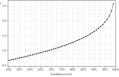
Figure 21: The relationship between the confidence level and the value of \(z\) in the formula for an approximate confidence interval.
The following figure is a repeat of figure 13. It shows confidence intervals based on the same estimated proportion, but with different confidence levels. The larger confidence levels lead to wider confidence intervals.
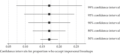
Figure 22: Confidence intervals from the same data, but with different confidence levels.
The distance from the sample estimate \(\hat{p}\) to the endpoints of the confidence interval is
\[ E = z \sqrt{\dfrac{\hat{p}(1-\hat{p})}{n}}. \]The quantity \(E\) is referred to as the margin of error. The margin of error is half the width of the confidence interval. Sometimes confidence intervals are reported as \(\hat{p} \pm E\); this means the bounds of the interval are not directly stated, but must be calculated.
We have seen in figure 22 that the margin of error is larger when the confidence level is larger. This is because the value of \(z\) from the standard Normal distribution will be larger when the confidence level is larger.
Example: Mobile-phone use among children
Continuing with the mobile-phone example, consider the 12–14 age group. Calculate an approximate 90% confidence interval for the true proportion of mobile-phone owners in this group.
Solution
From the table in the initial mobile-phone example, we have \(\hat{p} = \dfrac{918}{1250} = 0.734\). For a 90% confidence interval, we use \(z=1.64\), and so the margin of error is
\[ 1.64 \sqrt{\dfrac{0.734(1-0.734)}{1250}} = 0.0205. \]Hence, the 90% confidence interval is \(0.734 \pm 0.0205\), or \((0.714, 0.755)\). In percentage terms, the confidence interval is \(71.4\%\) to \(75.5\%\).
Exercise 6
Consider Casey's sample of Venus bars from exercise 5. He obtained a random sample of 180 wrappers, and found that 20 were winners. Rather than a 95% confidence interval for the true proportion of winning wrappers, consider a 99% confidence interval.
- Without calculating the 99% confidence interval, guess the lower and upper bounds.
- Find the value of the factor \(z\) from the standard Normal distribution for a 99% confidence interval (if necessary, by reading it off the graph in figure 21). Consider the ratio of the values of \(z\) for the 99% and 95% confidence intervals, and estimate the lower and upper bounds of the 99% confidence interval.
- Calculate the approximate 99% confidence interval for the true proportion of winning wrappers, based on Casey's sample of Venus bars.
- Consider Casey's suspicion that the true proportion of winners is not one in six. Comment on this, based on the 99% confidence interval.
Maximum margin of error
In the module Binomial distribution, we noted that if \(X \stackrel{\mathrm{d}}{=} \mathrm{Bi}(n,p)\), then the variance is largest (for a given value of \(n\)) when \(p = \dfrac{1}{2}\), in which case \(\mathrm{var}(X) = n \times \dfrac{1}{2} \times \dfrac{1}{2} = \dfrac{n}{4}\).
This has the direct consequence that, when estimating \(p\), the variance of \(\hat{P}\) is largest when \(p=0.5\), and is equal to \(\dfrac{0.25}{n}\). This is perhaps slightly unfortunate for political polling in particular, since such surveys are quite often estimating a characteristic (such as political preference) which is present in about half of the population.
However, there is some good news for the pollsters: While they may be in the realm of least precise inferences, they know how bad it can get. For a random sample of size \(n\), the standard deviation of \(\hat{P}\) cannot be bigger than \(\dfrac{0.5}{\sqrt{n}}\), and hence the margin of error for a 95% confidence interval is at most \(1.96\,\dfrac{0.5}{\sqrt{n}} = \dfrac{0.98}{\sqrt{n}}\).
To make the reporting of such polls succinct, this fact is sometimes exploited. The report simply uses the maximum margin of error for the given sample size \(n\), knowing that this is conservative: the precision will be as claimed if the estimated proportion \(\hat{p}\) is 0.5 (the percentage is 50%), and better than claimed otherwise.
Exercise 7
A Nielsen Poll published on 17 February 2013 reported that, in a two-party vote, 56% of voters prefer the Coalition (44% prefer ALP). The report indicates that the approximate margin of error is at most \(2.6\%\).
- Based on this margin of error, find the 95% confidence interval for the true proportion of voters preferring the Coalition. (Assume the margin of error provided is for a 95% level of confidence.)
- Based on this margin of error, approximately how many voters were surveyed?
- Why might Nielsen provide a single (maximum) margin of error in reporting on a variety of different outcomes (two-party-preferred vote, approval of the Prime Minister, approval of the Opposition Leader)?
- The approval of the Prime Minister was reported to be 40%. Find a 95% confidence interval for the true approval of the Prime Minister, based on the margin of error provided. Will this confidence interval be conservative (wider than it should be) or not (narrower than it should be)? Explain why.
When to use the Normal approximation
A guideline for when to use the Normal approximation for a confidence interval for \(p\) was given in the previous section: both \(x\) and \(n-x\) should be greater than 10. These conditions are generally met for the illustrative data in figure 23, based on \(n=100\).
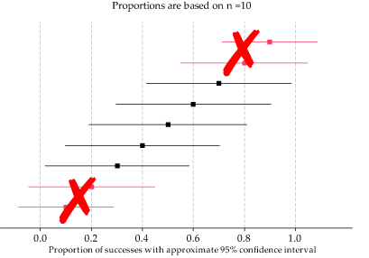
In contrast, the confidence intervals shown in figure 24 are based on data when \(n=10\); in no case is both \(x\) and \(n-x\) greater than 10. In four of the ten cases presented, the confidence intervals are nonsense: either the lower or the upper bound is outside the range 0 to 1. Of course, proportions must be in the range 0 to 1. This shows that these intervals are wrong, and it indicates that we should not trust the approximation when \(n\) is this small.
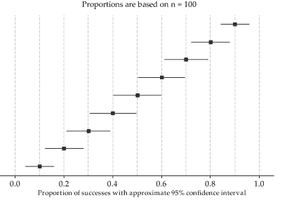
Figure 23: Approximate 95% confidence intervals for various estimates \(\hat{p}\), with \(n=100\).
Detailed description
Figure 24: Approximate 95% confidence intervals for various estimates \(\hat{p}\), with \(n=10\).
You may wonder whether it is possible to find a confidence interval for \(p\) when \(n\) is small, by avoiding the Normal approximation. The answer is that there is a method that uses only the binomial distribution, and does not approximate. It is beyond the scope of the curriculum.
Exercise 8
This exercise asks you to estimate \(\pi\), using a statistical approach. Suppose you were aware that the area of a circle is \(A = kr^2\), where \(r\) is the radius of the circle and \(k\) is a constant. Suppose you also knew that the equation for a circle centred at the origin is \(x^2 + y^2 = r^2\). So, you knew a lot about circles… but not the value of \(\pi\).
- Consider the unit square in the real plane, with corners at \((0,0)\), \((0,1)\), \((1,0)\) and \((1,1)\), and consider the circle of radius 1 centred at the origin. What proportion of the area of the square is covered by the circle, in terms of \(k\)? Define this proportion to be \(p\).
- Use the following approach to estimate \(p\), and hence \(k\).
- In an Excel spreadsheet, in columns A and B, store the variables \(x\) and \(y\). In each column, put \(10\ 000\) observations from the \(\mathrm{U}(0,1)\) distribution. Recall that this is achieved by entering \(\sf \text{=RAND()}\) in the first cell, and then filling down the column for \(10\ 000\) rows of data.
- In column C, calculate \(x^2 + y^2\).
- In column D, evaluate whether or not \(x^2 + y^2 < 1\), and store a '1' when this condition is satisfied, and a '0' otherwise.
- Use the \(10\ 000\) binary observations in column D to determine the proportion of the randomly generated points that are inside the circle. A simple way to do this is to average the values in column D. This is an estimate of \(p\).
- Report the point estimate and approximate 95% confidence interval for \(p\), based on this sample of size \(n=10\ 000\).
- In fact, as you will realise, in estimating \(p\) you have estimated \(\dfrac{\pi}{4} = 0.7854\). How precise is your estimate? Does your 95% confidence interval include the true value?
- Based on your 95% confidence interval for \(p\), what is your point estimate and approximate 95% confidence interval for \(k\)?
Next page - Content - Answers to exercises
| This publication is funded by the Australian Government Department of Education, Employment and Workplace Relations |
Contributors Term of use |