Content
More on the distribution of sample proportions
As in the previous sections, we are assuming that \(X \stackrel{\mathrm{d}}{=} \mathrm{Bi}(n,p)\). We have seen that the sample proportion \(\hat{P} = \frac{X}{n}\) is a random variable, and so has a distribution. We found that
\begin{align*} \mathrm{E}(\hat{P}) &= p \\ \mathrm{var}(\hat{P}) &= \frac{p(1-p)}{n} \\ \mathrm{sd}(\hat{P}) &= \sqrt{\frac{p(1-p)}{n}}. \end{align*}The fact that \(\mathrm{var}(\hat{P}) = \dfrac{p(1-p)}{n}\) illustrates that, for a given value of \(n\), the distribution of sample proportions will be more spread out when \(p\) is close to 0.5, and less spread out when \(p\) is close to 0 or 1. For example:
- if \(p=0.5\) and \(n=10\), then \(\hat{P}\) has variance 0.025 and standard deviation 0.1581
- if \(p=0.1\) and \(n=10\), or if \(p=0.9\) and \(n=10\), then \(\hat{P}\) has variance 0.009 and standard deviation 0.0949.
Exercise 1
The following table gives the standard deviation of \(\hat{P}\) for various values of \(p\) and \(n\). Complete the table by calculating the missing standard deviations, to two decimal places.
| \(n\) | \(p = 0.1\) | \(p = 0.3\) | \(p = 0.5\) | \(p = 0.7\) | \(p = 0.9\) |
|---|---|---|---|---|---|
| 10 | 0.09 | 0.16 | 0.09 | ||
| 50 | |||||
| 100 |
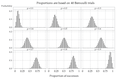
The dependence of the spread of the distribution of sample proportions on the true proportion \(p\) is illustrated in figure 6, where we consider the distribution of \(\hat{P} = \frac{X}{40}\), the proportion of successes from samples of size 40. figure 6 also shows that the distribution of sample proportions is more symmetric for values of \(p\) closer to 0.5.
Detailed description
Figure 6: True distributions of sample proportions \(\hat{P}\) for observations from the \(\mathrm{Bi}(40,p)\) distribution, for various values of \(p\).
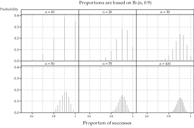
figure 7 shows six distributions of sample proportions based on varying sample size \(n\), but the same population parameter \(p=0.9\). As we saw in figure 5, as the sample size increases, there are more possible values for the sample proportion. Two other features of figure 7 are important. As we would expect, the spread of the distributions decreases as the sample size increases. Additionally, the symmetry of the distributions increases with sample size.
Detailed description
Figure 7: True distributions of sample proportions \(\hat{P}\) for observations from the \(\mathrm{Bi}(n,0.9)\) distribution, for various values of \(n\).
The distribution of sample proportions for large sample sizes
What does the distribution of the sample proportion look like when the sample size is large? As we have seen in figure 7, even when \(p\) is as large as 0.9, if the sample size \(n\) is large, the distribution of \(\hat{P}\) looks quite symmetric: Look at the three distributions in the second row, for \(n=50\), \(n=75\) and \(n=100\).
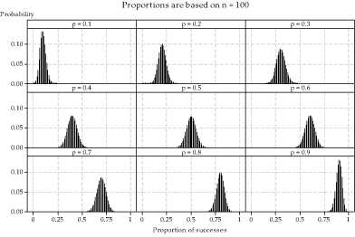
In figure 8, a sample size of \(n=100\) has been used throughout. With this large sample size, the distributions across the range of true proportions from 0.1 to 0.9 are quite symmetric, and clearly much more symmetric than the examples we have seen in previous figures when \(n\) is not large. With the large number of possibilities for the sample proportion (101 different values), the distributions are reminiscent of a continuous distribution. The shape of each distribution is symmetric, and like a Normal distribution. Of course, the distribution cannot actually be a Normal distribution, because the Normal distribution is continuous, and the distribution of sample proportions is discrete. But visually it appears that a Normal distribution would be quite a good approximation. This visual impression is correct, as we now demonstrate.
Detailed description
Figure 8: True distributions of sample proportions \(\hat{P}\) for observations from the \(\mathrm{Bi}(100,p)\) distribution, for various values of \(p\).
Detailed description
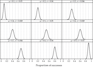
Figure 9: Normal distributions with means and standard deviations corresponding to those of the distributions of sample proportions in figure 8.
The nine Normal distributions shown in figure 9 have means and standard deviations corresponding to those of the distributions of sample proportions in figure 8. For example, the top-left panel in figure 8 shows the distribution of \(\hat{P}\) for \(n=100\) and \(p=0.1\), so \(\mathrm{E}(\hat{P}) = p = 0.1\) and \(\mathrm{sd}(\hat{P}) = \sqrt{\frac{p(1-p)}{n}} = 0.03\). Hence, the top-left Normal distribution in figure 9 has mean \(\mu = 0.1\) and standard deviation \(\sigma = 0.03\).
These two figures illustrate how the distribution of sample proportions can be approximated by a Normal distribution for large sample sizes.
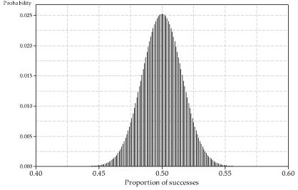
figure 10 shows the distribution of sample proportions based on \(n=1000\) and \(p=0.5\). Here we see an even closer approximation to 'continuity' and a Normal distribution. Again, the distribution cannot actually be Normal, because the proportions can only take discrete values. But consider how close together the discrete values now are, when \(n\) is so large. The gaps between the spikes (representing the probabilities) are only 0.001 apart, because the proportions can take values such as \(0.500, 0.501, 0.502, \dots\). So the appearance of a Normal distribution is stronger than any of the examples we have seen for smaller sample sizes.
Detailed description
Figure 10: Distribution of the sample proportion \(\hat{P}\) from the \(\mathrm{Bi}(1000,0.5)\) distribution.
The Normal approximation described here is used later, when we obtain an approximate confidence interval for the unknown \(p\), based on an observation from the binomial distribution \(\mathrm{Bi}(n,p)\), for large \(n\). Before getting to the practicalities, however, we consider some very important general ideas about confidence intervals.
Next page - Content - Confidence intervals
| This publication is funded by the Australian Government Department of Education, Employment and Workplace Relations |
Contributors Term of use |