Content

The sample proportion as a random variable

The module Random sampling includes the example of making observations on the \(\mathrm{Bi}(10,0.5)\) distribution. This example is motivated by supposing that, in the population of voters, 50% prefer the Labor party, and then looking at what happens for many small samples of 10 voters.

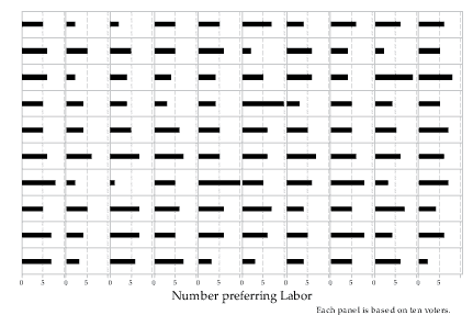
If we count the number of Labor voters in one sample of 10 voters, we have an observation from the binomial distribution with parameters \(n=10\) and \(p=0.5\). If we do this 100 times, we have 100 observations from this binomial distribution. An example of 100 actual observations is shown in figure 2; the number of people preferring Labor is shown as a horizontal bar.

Detailed description

Figure 2: 100 observations from the \(\mathrm{Bi}(10,0.5)\) distribution.

In figure 3, the same 100 observations are represented, but the proportion preferring Labor is plotted, rather than the number. As each binomial observation is based on a random sample of 10 voters, the top part of figure 3 is simply a re-scaling of figure 2 with the number preferring Labor divided by 10 to provide the proportion.

Detailed description

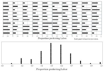
Figure 3: 100 proportions based on observations from the \(\mathrm{Bi}(10,0.5)\) distribution.

The bottom part of figure 3 provides an alternative representation of the same 100 observations. Each observed proportion is plotted as a dot, and the dots are stacked up when there are multiple observations of the same value.

For example, you can see that there is one dot at 0.1, and you should be able to find the corresponding single sample with a proportion of \(\frac{1}{10} = 0.1\) in the top part of figure 3. Similarly, there are two dots at 1.0, corresponding to the two samples with a proportion of \(\frac{10}{10} = 1.0\) in the top part of figure 3.

Since the observations shown in figure 3 are taken from a binomial distribution with \(p=0.5\), it is not surprising to find that the most frequently observed sample proportion among the 100 cases is 0.5.

Figures 2 and 3 are based on observations from the binomial distribution with \(n=10\) and \(p=0.5\). What about the distribution itself?

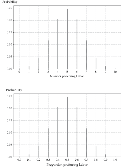
The top part of figure 4 shows this binomial distribution. Assuming that this is an appropriate model for the number of people preferring Labor in a sample of 10 voters, the probability of five people preferring Labor is about 0.25 (it is 0.2461 to four decimal places). We can think of this as meaning that, in the long run, among many samples of size 10, the proportion of samples in which five voters prefer Labor will be \(24.61\%\).

Detailed description

Figure 4: The \(\mathrm{Bi}(10,0.5)\) distribution (top), and the distribution of sample proportions for observations from the \(\mathrm{Bi}(10,0.5)\) distribution (bottom).

The top part of figure 4 corresponds closely to the bottom part; the latter shows the true distribution of sample proportions, each based on an observation from the \(\mathrm{Bi}(10,0.5)\) distribution. The distribution in the bottom part is the same shape as the \(\mathrm{Bi}(10,0.5)\) distribution in the top part; it is not the \(\mathrm{Bi}(10,0.5)\) distribution because it has a different scale on the horizontal axis — the scale based on proportions.

Think about the distribution shown in the bottom part of figure 4 some more. It tells us about the true pattern of repeated sample proportions based on observations from \(\mathrm{Bi}(10,0.5)\). About one quarter of the sample proportions will be 'right on the money': they will be exactly equal to the true population proportion, \(p=0.5\). If the sample proportion is not exactly 0.5, it is quite likely that it is close to 0.5: the next most likely sample proportions are 0.4 and 0.6 (equally likely).

It is unlikely that the sample proportion will be a long way from the true proportion. The worst possible outcomes (furthest from the population proportion \(p=0.5\)) are sample proportions of \(\frac{0}{10} = 0\) or \(\frac{10}{10} = 1\). They have a very small probability of occurring. Each of the outcomes 0 and 1 has probability equal to 0.0010. They are not going to occur very often, in the long run. And after all, when we looked at 100 sample proportions, none of them was equal to 0, and only two of them were equal to 1 (figure 3).

All of this shows us that the sample proportion \(\hat{P} = \frac{X}{n}\) is itself a random variable. In a sense, this is obvious, since it follows directly from its definition: it is a simple function of the binomial random variable \(X\). So \(\hat{P}\) has a distribution. It has a mean and a variance: what are they?

Mean and variance of the sample proportion

We will use the following general result about the mean and variance of a linear transformation of a random variable.

If \(X\) is a discrete random variable and \(Y = aX + b\), then

• \(\mathrm{E}(Y) = a\,\mathrm{E}(X) + b\)
• \(\mathrm{var}(Y) = a^2\,\mathrm{var}(X)\)
• \(\mathrm{sd}(Y) = |a|\,\mathrm{sd}(X)\).

The first part is proved in the module Discrete probability distributions. The second part can be proved using a similar approach, and then the third part follows.

Now assume that \(X \stackrel{\mathrm{d}}{=} \mathrm{Bi}(n,p)\). From the module Binomial distribution, we know that \(\mathrm{E}(X) = np\) and \(\mathrm{var}(X) = np(1-p)\). It follows that

\[ \mathrm{E}(\hat{P}) = \mathrm{E}\Bigl(\frac{X}{n}\Bigr) = \frac{1}{n}\, \mathrm{E}(X) = \frac{1}{n} \times np = p. \]

So the distribution of the sample proportion \(\hat{P}\) is centred around \(p\). For statistical inference, this is highly desirable. It means that in the long run, on average, the sample proportion will neither over-estimate nor under-estimate the true value of \(p\). Of course, a specific estimate will be out by a bit; but in the long run, the estimates average out to the true proportion \(p\).

What about the variance? Using the general result above:

\begin{align*} \mathrm{var}(\hat{P}) &= \mathrm{var}\Bigl(\frac{X}{n}\Bigr) \\ &= \Bigl(\frac{1}{n}\Bigr)^2 \mathrm{var}(X) \\ &= \frac{1}{n^2}\, np(1-p) \\ &= \frac{p(1-p)}{n}. \end{align*}

It follows that the standard deviation of \(\hat{P}\) is given by

\[ \mathrm{sd}(\hat{P}) = \sqrt{\frac{p(1-p)}{n}}. \]

The presence of \(n\) in the denominator of the variance of the sample proportion \(\hat{P}\) is very important. It means that, for larger samples, the spread of the distribution of \(\hat{P}\) will be smaller. This is a good thing: Since the distribution is centred on \(p\), the smaller the variance, the more likely it is that sample proportions will be close to \(p\). We explore this further in the section More on the distribution of sample proportions.

In summary, for population proportion \(p\) and sample size \(n\), the mean, variance and standard deviation of the sample proportion \(\hat{P}\) are as follows:

\begin{align*} \mathrm{E}(\hat{P}) &= p \\ \mathrm{var}(\hat{P}) &= \frac{p(1-p)}{n} \\ \mathrm{sd}(\hat{P}) &= \sqrt{\frac{p(1-p)}{n}}. \end{align*}

To illustrate these results, we look at what happens in our voting-preference example when we increase the sample size from 10 voters to 100 voters.

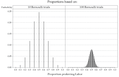
figure 5 shows the distribution of sample proportions based on observations from the \(\mathrm{Bi}(n,0.5)\) distribution for \(n=10\) and for \(n=100\). When \(n=100\), there are 101 possible values for the proportion of people voting Labor.

Notice what has changed between \(n=10\) and \(n=100\), and also what has not changed. What has not changed is that the distribution of the sample proportion \(\hat{P}\) is still centred around the population proportion \(p=0.5\). This is true for any value of \(n\). What has changed is that, for \(n=100\), the distribution is much more narrowly concentrated around the mean \(p=0.5\). When \(n=100\), it is more likely that a sample proportion will be close to \(p=0.5\), compared to when \(n=10\).

Detailed description

Figure 5: True distributions of sample proportions for observations from the \(\mathrm{Bi}(10,0.5)\) distribution (left) and the \(\mathrm{Bi}(100,0.5)\) distribution (right).

We have discussed the sample proportion \(\hat{P}\) as providing a point estimate of \(p\). We now develop this idea further, moving towards making a detailed inference about \(p\): finding an interval which we are 'confident' contains \(p\).

Next page - Content - Population parameters and sample estimates