Content

Normal distribution

The Normal distribution is arguably the most important continuous distribution. It is used throughout the sciences, because of a remarkable result known as the central limit theorem, which is covered in the module Inference for means. Due to the phenomenon behind the central limit theorem, many variables tend to show an empirical distribution that is close to the Normal distribution.

If \(X\) has a Normal distribution with mean \(\mu\) and standard deviation \(\sigma\), then we write that \(X \stackrel{\mathrm{d}}{=} \mathrm{N}(\mu,\sigma^2)\); the probability density function of \(X\) is given by

\[ f_X(x) = \dfrac{1}{\sigma \sqrt{2\pi}} \exp\Bigl(\dfrac{-(x-\mu)^2}{2\sigma^2}\Bigr), \qquad\text{for } x \in \mathbb{R}. \]

This distribution is so important that it is well known in general culture, where it is often referred to as the bell curve — for example, in the controversial 1994 book by R. J. Herrnstein entitled The Bell Curve: Intelligence and Class Structure in American Life.

Detailed description

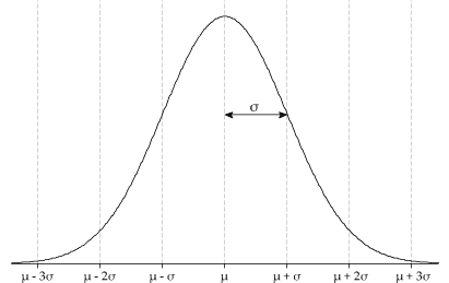
Figure 2: The pdf of a Normal random variable with mean \(\mu\) and standard deviation \(\sigma\).

Several properties of the Normal distribution are worth noting:

• It is easy to see from the formula for \(f_X(x)\) that the distribution is symmetric around \(x = \mu\). By the properties of the mean, this confirms that \(\mu_X = \mathrm{E}(X) = \mu\).
• The pdf has one peak, which is at \(x = \mu\).
• The pdf has two points of inflexion, where the second derivative of the pdf changes sign. They are at \(x = \mu-\sigma\) and \(x = \mu+\sigma\); see figure 2. This is very useful when we need to graph a Normal pdf with a given \(\mu\) and \(\sigma\): we can use \(\mu\) to position the curve correctly, and \(\sigma\) to get the scale right.
  
  When drawing the bell-shaped curve, it can sometimes be easier to write the value of \(\mu\) on the \(x\)-axis, annotate the pdf with the value of \(\sigma\) for the distance between \(\mu\) and \(\mu+\sigma\), and then fill in the scale on the \(x\)-axis. At the very least, it is helpful to show the actual value of \(\sigma\) on the plot, when thinking about a practical application.
• For the Normal distribution: \begin{align*} \Pr(\mu - \sigma \leq X \leq \mu+\sigma) &= 0.6827 \\\\ \Pr(\mu - 2\sigma \leq X \leq \mu+2\sigma) &= 0.9545 \\\\ \Pr(\mu - 3\sigma \leq X \leq \mu+3\sigma) &= 0.9973. \end{align*} These probabilities are often thought of more approximately as 68.3%, 95.4% and 99.7%, or even as 68%, 95% and 99.7%; they are illustrated in figure 3.

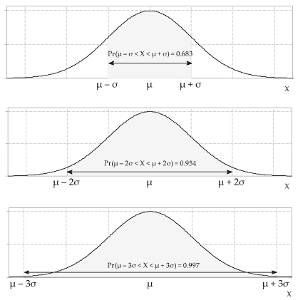
Figure 3: Probabilities of three intervals for the Normal distribution.

Recall that, for continuous random variables, it is the cumulative distribution function (cdf) and not the pdf that is used to find probabilities, because we are always concerned with the probability of the random variable being in an interval.

Before considering the cdf of \(X \stackrel{\mathrm{d}}{=} \mathrm{N}(\mu,\sigma^2)\), we explore a very useful feature of the Normal distribution.

A random variable with the standard Normal distribution, commonly denoted by \(Z\), has mean zero and standard deviation one. That is, \(Z \stackrel{\mathrm{d}}{=} \mathrm{N}(0,1)\). The pdf for the standard Normal distribution is

\[ f_Z(z) = \dfrac{1}{\sqrt{2\pi}} \exp\bigl(-\tfrac{1}{2} z^2\bigr), \qquad\text{for } z \in \mathbb{R}. \]

The probabilities for any Normal distribution can be reduced to probabilities for the standard Normal distribution, using the device of standardisation. Therefore probability calculations for any Normal distribution can be reduced to calculations for the standard Normal distribution, as shown by the following result.

Standardisation of a Normal distribution

If \(X \stackrel{\mathrm{d}}{=} \mathrm{N}(\mu,\sigma^2)\) and \(X_s = \dfrac{X-\mu}{\sigma}\), then \(X_s \stackrel{\mathrm{d}}{=} \mathrm{N}(0,1)\).

Proof

Finding probabilities for the standard Normal distributions requires technology: the cdf of \(Z \stackrel{\mathrm{d}}{=} \mathrm{N}(0,1)\) is

\[ F_Z(z) = \int_{-\infty}^z \dfrac{1}{\sqrt{2\pi}} \exp\bigl(-\tfrac{1}{2}t^2\bigr) \;dt. \]

This integral does not have a closed form, and must be evaluated using numerical integration. It is available in statistical software, on many calculators, in Matlab and in Excel; here we describe the Excel function. It is \(\sf \text{NORM.S.DIST}\), which requires two arguments:

1. the value of \(z\) for which the cdf is required
2. a true/false (or equivalently, 1/0) argument that controls whether the cdf (argument equals \(\sf \text{TRUE}\) or \(\sf \text{1}\)) or pdf (argument equals \(\sf \text{FALSE}\) or \(\sf \text{0}\)) is returned.

For example, to use Excel to find the value of \(F_Z(1.5)\), the cdf of the standard Normal distribution when \(z=1.5\), enter

\[ \sf \text{=NORM.S.DIST(1.5, 1)} \]

in a cell and hit return. You should obtain the value 0.9332.

Note that, in this example, \(31\;000 = \mu + \sigma\) and \(36\;000 = \mu + 2 \sigma\). If the mean and the standard deviation were different from these, but we still sought the probability of being between one and two standard deviations greater than the mean, then the same probability would be obtained. This is illustrated in figure 4, in which the same probability as that obtained in the example (\(0.1359\)) is found in all four cases.

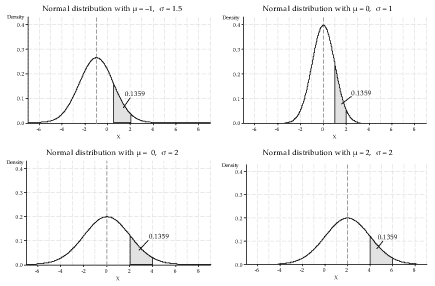
Detailed description

Figure 4: Four Normal probability density functions.

Interactive 1   Interactive 2

The cdf of any Normal distribution can also be found, using technology, without first standardising. If \(X \stackrel{\mathrm{d}}{=} \mathrm{N}(\mu,\sigma^2)\), then the cdf of \(X\) is given by

\[ \Pr(X \leq x) = F_X(x) = \int_{-\infty}^x \dfrac{1}{\sigma \sqrt{2\pi}} \exp\Bigl(\dfrac{-(t-\mu)^2}{2\sigma^2}\Bigr) \;dt, \qquad\text{for } x \in \mathbb{R}. \]

One way to obtain this is in Excel using the function \(\sf \text{NORM.DIST}\). This function requires four arguments:

1. the value of \(x\) for which the cdf should be evaluated
2. the mean \(\mu\)
3. the standard deviation \(\sigma\)
4. a true/false (or equivalently, 1/0) argument that controls whether the cdf (argument equals \(\sf \text{TRUE}\) or \(\sf \text{1}\)) or pdf (argument equals \(\sf \text{FALSE}\) or \(\sf \text{0}\)) is returned.

We can use this function to find the required probabilities in the crowd-size example directly. For example, you should find that typing

\[ \sf \text{=NORM.DIST(36000, 26000, 5000, 1)} \]

returns the value 0.9772.

Sometimes we need to find a quantile of the Normal distribution. Let \(q\) be a number between 0 and 1. Then the \(q\) quantile, \(c_q\), of the Normal distribution with cdf \(F_X\) is defined by the equation

\[ F_X(c_q) = q. \]

To obtain the value of \(c_q\), we can use technology. In Excel, for example, the function is \(\sf \text{NORM.INV}\). It requires three arguments:

1. the value of \(q\) for which the inverse cdf should be evaluated
2. the mean \(\mu\)
3. the standard deviation \(\sigma\).

We shall study confidence intervals in the two modules Inference for proportions and Applications of differentiation. In that context, we want to know the bounds of the central 95% of the distribution for \(Z \stackrel{\mathrm{d}}{=} \mathrm{N}(0,1)\). That is, we want \(z\) such that

\[ \Pr(-z < Z < z) = 0.95. \]

We can find this \(z\) using the same techniques as for quantiles.

Since the standard Normal distribution is symmetric about 0, we require

\[ \Pr(Z \leq -z) = \tfrac{1}{2}(1 - 0.95) = 0.025 \qquad\text{and}\qquad \Pr(Z \geq z) = \tfrac{1}{2}(1 - 0.95) = 0.025. \]

So we want

\[ F_Z(z) = \Pr(Z \leq z) = 1 - 0.025 = 0.975. \]

We can now find \(z\) in Excel using

\[ \sf \text{=NORM.INV(0.975, 0, 1)}, \]

which gives 1.96. This is illustrated in the following figure.

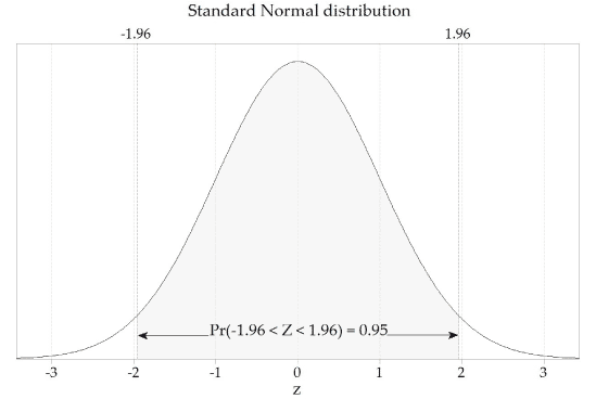
Figure 5: The standard Normal distribution, \(Z \stackrel{\mathrm{d}}{=} \mathrm{N}(0,1)\).

More generally, if we are given a probability \(p\) and we want \(z\) with \(\Pr(-z < Z < z) = p\), then we find \(z\) such that

\[ F_Z(z) = \dfrac{p+1}{2}. \]

Next page - Answers to exercises