Content
Exponential distribution
The exponential distribution is defined as follows. Suppose that the continuous random variable \(T\) has an exponential distribution with rate \(\alpha > 0\), which we write as \(T \stackrel{\mathrm{d}}{=} \exp(\alpha)\). Then \(T\) has the following pdf:
\[ f_T(t) = \begin{cases} \alpha e^{-\alpha t} &\text{if } t > 0, \\\\ 0 &\text{otherwise.} \end{cases} \]Four exponential pdfs are shown in figure 1 on the same scale. Note that they all have the same shape. The greater the rate \(\alpha\), the more likely it is that the corresponding exponential random variable takes a small value. This makes sense: if the events are occurring at a high rate, it will tend to be a short time until the first event, and vice versa.
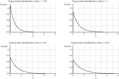
Figure 1: Four exponential probability density functions with different values of \(\alpha\).
An exponential random variable can be regarded as the waiting time until the first event in a Poisson process with rate \(\alpha\). The curriculum does not cover Poisson processes, so we need to describe them briefly here. It is appropriate to think of a 'random process' in which events occur in time, independently of each other, at a rate per unit time. This means that processes that are systematic (such as train timetables) or approximately regular (the arrival of waves on a beach) are not Poisson processes. Examples of phenomena that might be suitably modelled with this distribution include:
- radioactive decay
- the occurrences of a rare disease in a large population
- arrival of a packet of information on the internet.
Example: Country hospital
Let \(T\) be the interval between births at a country hospital, for which the average time between births is seven days. We assume the distribution of the time between births follows an exponential distribution. Clearly, multiple births (twins, triplets, \ldots) will violate the assumption of independence; we deal with this by defining a 'birth' to be a birth event for one mother, regardless of the number of babies born. The unit of time is 'day', and the corresponding average rate of events is one birth every seven days, so that \(\alpha = \dfrac{1}{7}\). Hence, \(T \stackrel{\mathrm{d}}{=} \exp(\dfrac{1}{7})\) and
\[ f_T(t) = \begin{cases} \dfrac{1}{7} e^{-\dfrac{1}{7} t} &\text{if } t > 0, \\\\ 0 &\text{otherwise.} \end{cases} \]We now consider some of the characteristics of the exponential distribution.
Mean of the exponential distribution
If \(T \stackrel{\mathrm{d}}{=} \exp(\alpha)\), then \(\mu_T = \mathrm{E}(T) = \dfrac{1}{\alpha}\).
Proof
We have
\begin{align*} \mathrm{E}(T) &= \int_0^\infty t\,f_T(t) \;dt \\\\ &= \int_0^\infty t \alpha e^{-\alpha t} \;dt \\\\ &= \bigl[-t e^{-\alpha t}\bigr]_0^\infty + \int_0^\infty e^{-\alpha t} \,dt \qquad \text{(using integration by parts)} \\\\ &= 0 - 0 + \bigl[-\tfrac{1}{\alpha} e^{-\alpha t} \bigr]_0^\infty \\\\ &= 0 + \tfrac{1}{\alpha} \\\\ &= \tfrac{1}{\alpha}. \end{align*}\(\Box\)
The proof for the variance also uses integration by parts; it is not provided here.
Variance of the exponential distribution
If \(T \stackrel{\mathrm{d}}{=} \exp(\alpha)\), then \(\mathrm{var}(T) = \dfrac{1}{\alpha^2}\).
The cdf of \(T\) is given by
\[ \Pr(T \leq t) = F_T(t) = \int_{-\infty}^{t} f_T(u) \;du. \]So, for \(t \leq 0\), we have \(F_T(t) = 0\), and for \(t > 0\), we have
\[ F_T(t) = \int_0^t \alpha e^{-\alpha u} \;du = \bigl[-e^{-\alpha u}\bigr]_0^t = 1 - e^{-\alpha t}. \]Hence, we can write the cdf of \(T\) as
\[ \Pr(T \leq t) = F_T(t) = \begin{cases} 0 &\text{if } t \leq 0, \\\\ 1 - e^{-\alpha t} &\text{if } t > 0. \end{cases} \]An obvious consequence of the cdf having this form is that the probability of the waiting time \(T\) exceeding \(t\) is
\[ \Pr(T > t) = e^{-\alpha t}, \qquad\text{for } t > 0. \]Example: Country hospital, continued
We return to the example of births at a country hospital, in which we assume that the time between successive births, \(T\), has an exponential distribution with rate \(\dfrac{1}{7}\); that is, \(T \stackrel{\mathrm{d}}{=} \exp(\dfrac{1}{7})\). Hence, we have
- \(\mu_T = \mathrm{E}(T)\) = 7 days
- \(\sigma^2_T = \mathrm{var}(T)\) = 49
- \(\sigma_T = \mathrm{sd}(T)\) = 7 days.
What is the chance that there is a birth in the next 10 days? 10 hours? 10 minutes?
In general, the chance of a birth in the next \(t\) days is
\[ F_T(t) = 1 - e^{-\dfrac{1}{7} t}, \qquad\text{for } t>0. \]The unit of time being used here is days. The probability that the waiting time until the next birth is less than or equal to 10 days is therefore
\begin{align*} F_T(10) &= 1 - \exp\bigl(-\tfrac{10}{7}\bigr) \\\\ &= 1 - e^{-1.429} = 1 - 0.240 = 0.760. \end{align*}Ten hours equals \(\dfrac{5}{12}\) days. The probability that the waiting time until the next birth is less than or equal to 10 hours is therefore
\begin{align*} F_T\bigl(\tfrac{5}{12}\bigr) &= 1 - \exp\bigl(-\tfrac{1}{7} \times \tfrac{5}{12}\bigr) \\\\ &= 1 - e^{-0.060} = 0.058. \end{align*}Finally, note that 10 minutes equals \(\dfrac{1}{144}\) days, so the probability that the waiting time until the next birth is less than or equal to 10 minutes is
\begin{align*} F_T\bigl(\tfrac{1}{144}\bigr) &= 1 - \exp\bigl(-\tfrac{1}{7} \times \tfrac{1}{144}\bigr) \\\\ &= 1 - e^{-0.00099} = 0.00099. \end{align*}Note that, for small values of \(k\), we have \(1 - e^{-k} \approx 1 - (1 - k) = k\). Hence, if \(\alpha t\) is small, then the chance of an event before time \(\alpha t\) is approximately equal to \(\alpha t\). This approximation applies to the second and third cases here.
An intriguing feature of the exponential distribution is its lack of memory property. Roughly speaking, it is as the name suggests: the process 'does not remember what has happened up until now' and the distribution of the waiting time, given that it has already exceeded some amount of time \(t_0\), has the same exponential-distribution form, just translated by \(t_0\).
The lack of memory property is quite readily established. For \(t_0 > 0\) and \(t > t_0\):
\begin{alignat*}{2} \Pr(T > t \mid T > t_0) &= \dfrac{\Pr(T > t \text{ and } T > t_0)}{\Pr(T > t_0)} &\qquad&(\text{rule for conditional probability}) \\\\ &= \dfrac{\Pr(T > t)}{\Pr(T > t_0)} &&(\text{since } \text{''} T > t \text{''} \subseteq \text{''} T > t_0 \text{''}) \\\\ &= e^{-\alpha(t - t_0)}. \end{alignat*}Exercise 1
Suppose that the time between emergency calls to a small suburban fire station follows an exponential distribution with an average rate of 1.8 calls per day.
- Phil the fireman has just clocked on. What is the chance of a call in the next 15 minutes?
- Phil has nearly finished his shift: 15 minutes to go. There has been no call during his shift so far. What is the chance of a call in the next 15 minutes?
- Judy works a \(10\)-hour shift, Mondays to Thursdays. What is the probability that she has no calls in a shift?
- What is the probability that she has no calls in four successive days?
- Judy is talking about her job: 'In 10% of shifts, there's a call in the first \(x\) hours of the shift.' What is \(x\), to one decimal place?
Next page - Content - Normal distribution
| This publication is funded by the Australian Government Department of Education, Employment and Workplace Relations |
Contributors Term of use |