Content
Cumulative distribution functions
The cumulative distribution function (cdf) of any random variable \(X\) is the function \(F_X \colon \mathbb{R} \to [0,1]\) defined by
\[ F_X(x) = \Pr(X \leq x). \]Both discrete and continuous random variables have cdfs, although we did not focus on them in the modules on discrete random variables and they are more straightforward to use for continuous random variables.
As noted in the module Discrete probability distributions , the use of lower case \(x\) as the argument is arbitrary here: if we wrote \(F_X(t)\), it would be the same function, determined by the random variable \(X\). But it helps to associate the corresponding lower-case letter with the random variable we are considering.
The cdf is defined for all real values \(x\), sometimes implicitly rather than explicitly. In the example in the previous section, we considered the random variable \(T_i\), the total time spent on Facebook by individual \(i\) up to age 18. This is a measurement of time, in years, which must be between 0 and 18. So we know that the cdf of \(T_i\) must be zero for any value of \(t<0\). That is, if \(t<0\), then \(F_{T_i}(t) = \Pr(T_i \leq t) = 0\). At the other extreme, we know that \(T_i\) must be less than or equal to 18. So, if \(t\geq 18\), then \(F_{T_i}(t) = \Pr(T_i \leq t) = 1\).
Remember that outcomes for random variables define events in the event space, which is why we are able to assign probabilities to such outcomes. Let \(X\) be a random variable with cdf \(F_X(x)\). For \(a<b\), we can consider the following events:
- \(C =\) ''\(X \leq a\)''
- \(D =\) ''\(a < X \leq b\)''
- \(E =\) ''\(X \leq b\)''.
Then \(C\) and \(D\) are mutually exclusive, and their union is the event \(E\). By the third axiom of probability, this tells us that
\begin{alignat*}{2} && \Pr(E) &= \Pr(C) + \Pr(D) \\\\ &\implies\quad & \Pr(X \leq b) &= \Pr(X \leq a) + \Pr(a < X \leq b) \\\\ &\implies & \Pr(a < X \leq b) &= \Pr(X \leq b) - \Pr(X \leq a) \\\\ &\implies & \Pr(a < X \leq b) &= F_X(b) - F_X(a). \end{alignat*}The cumulative distribution function \(F_X(x)\) of a random variable \(X\) has three important properties:
- The cumulative distribution function \(F_X(x)\) is a non-decreasing function. This follows directly from the result we have just derived: For \(a < b\), we have \[ \Pr(a < X \leq b) \geq 0 \ \implies\ F_X(b) - F_X(a) \geq 0 \ \implies\ F_X(a) \leq F_X(b). \]
- As \(x \to -\infty\), the value of \(F_X(x)\) approaches 0 (or equals 0). That is, \(\lim\limits_{x\to-\infty} F_X(x) = 0\). This follows in part from the fact that \(\Pr(\varnothing) = 0\).
- As \(x \to \infty\), the value of \(F_X(x)\) approaches 1 (or equals 1). That is, \(\lim\limits_{x\to\infty} F_X(x) = 1\). This follows in part from the fact that \(\Pr(\mathcal{E}) = 1\).
All of the above discussion applies equally to discrete and continuous random variables.
We now turn specifically to the cdf of a continuous random variable. Its form is something like that shown in the following figure. We require a continuous random variable to have a cdf that is a continuous function.
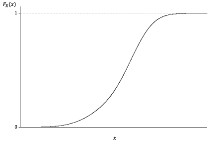
Detailed description
Figure 1: The general appearance of the cumulative distribution function of a continuous random variable.
We now use the cdf a continuous random variable to start to think about the question of probabilities for continuous random variables. For discrete random variables, probabilities come directly from the probability function \(p_X(x)\): we identify the possible discrete values that the random variable \(X\) can take, and then specify somehow the probability for each of these values.
For a continuous random variable \(X\), once we know its cdf \(F_X(x)\), we can find the probability that \(X\) lies in any given interval:
\[ \Pr(a < X \leq b) = F_X(b) - F_X(a). \]But what if we are interested in the probability that a continuous random variable takes a specific single value? What is \(\Pr(X=x)\) for a continuous random variable?
We can address this question by considering the probability that \(X\) lies in an interval, and then shrinking the interval to a single point. Formally, for a continuous random variable \(X\) with cdf \(F_X(x)\):
\begin{alignat*}{2} \Pr(X = x) &\leq \lim_{h \to 0^+} \Pr(x - h < X \leq x) \\\\ &= \lim_{h \to 0^+} \bigl(F_X(x) - F_X(x-h)\bigr) \\\\ &= F_X(x) - F_X(x) &\qquad&(\text{since } F_X \text{ is continuous}) \\\\ &= 0. \end{alignat*}Hence, \(\Pr(X = x) = 0\). This is a somewhat disconcerting result: It seems to be saying that we can never really observe a continuous random variable taking a specific value, since the probability of observing any value is zero.
In fact, this is true. Continuous random variables are really abstractions: what we observe is always rounded in some way. It helps to think about some specific cases.
Example: Random numbers
Suppose we consider real numbers randomly chosen between 0 and 1, for which we record \(X_1\), the random number truncated to one decimal place. For example, the number 0.07491234008 is recorded as 0.0 (as the first decimal place is zero). Note that this means we are not rounding, but truncating. If the mechanism generating these numbers has no preference for any position in the interval \((0,1)\), then the distribution of the numbers we obtain will be such that
\[ \Pr(X_1 = 0.0) = \Pr(X_1 = 0.1) = \dots = \Pr(X_1 = 0.9) = \tfrac{1}{10}. \]This is a discrete random variable, with the same probability for each of the ten possible outcomes.
Now suppose that instead we record \(X_2\), the random number truncated to two decimal places (again, not rounding). For example, if the real number is \(0.9790295134\), we record 0.97. This random variable is also discrete, with
\[ \Pr(X_2 = 0.00) = \Pr(X_2 = 0.01) = \dots = \Pr(X_2 = 0.99) = \tfrac{1}{100}. \]The distributions of \(X_1\) and \(X_2\) are shown in figure 2.
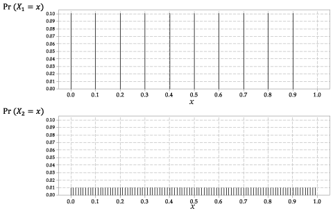
Figure 2: The probability functions \(p_{X_1}(x)\) for \(X_1\) and \(p_{X_2}(x)\) for \(X_2\).
You can see where this is going: If we record the first \(k\) decimal places, the random variable \(X_k\) has \(10^k\) possible outcomes, each with the same probability \(10^{-k}\).
Excel has a function that produces real numbers between 0 and 1, chosen so that there is no preference for any position in the interval \((0,1)\). If you enter \(\sf \text{=RAND()}\) in a cell and hit return, you will obtain such a number. Increase the number of decimal places shown in the cell. Keep going until you get a lot of zeroes on the end of the number; you might need to increase the size of the cell. Your spreadsheet should look like figure 3, although of course the specific number will be different… it is random, after all!
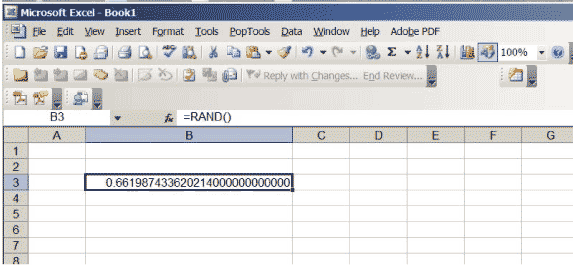
Figure 3: An Excel spreadsheet with a random number from between 0 and 1.
If you hit the key 'F9' repeatedly at this point, you will see a sequence of random numbers, all between 0 and 1. From examining these, it appears that Excel actually produces observations on the random variable \(X_{15}\), the first 15 decimal places of the number. So the chance of any specific one of these numbers occurring is \(10^{-15}\).
Now consider the chance that each of these discrete random variables \(X_1, X_2, X_3, \dots\) takes a value in the interval \([0.3,0.4)\), for example. We have
\begin{align*} \Pr(0.3 \leq X_1 < 0.4) &= \Pr(X_1 = 0.3) = 0.1, \\\\ \Pr(0.3 \leq X_2 < 0.4) &= \Pr(X_2 = 0.30) + \Pr(X_2 = 0.31) + \dots + \Pr(X_2 = 0.39) \\\\ &= 10 \times 0.01 = 0.1, \\\\ \Pr(0.3 \leq X_3 < 0.4) &= 10^2 \times 10^{-3} = 0.1, \\\\ \Pr(0.3 \leq X_4 < 0.4) &= 10^3 \times 10^{-4} = 0.1, \\\\ &\vdots \\\\ \Pr(0.3 \leq X_k < 0.4) &= 10^{k-1} \times 10^{-k} = 0.1, \\\\ & \vdots \end{align*}As we make the distribution finer and finer, with more and more possible discrete values, the probability that any of these discrete random variables lies in the interval \([0.3,0.4)\) is always 0.1.
As \(k\) increases, the discrete random variable \(X_k\) can be thought of as a closer and closer approximation to a continuous random variable. This continuous random variable, which we label \(U\), has the property that
\[ \Pr(a \leq U \leq b) = b - a, \qquad\text{for } 0 \leq a \leq b \leq 1. \]For example, \(\Pr(0.3 \leq U \leq 0.4) = 0.4 - 0.3 = 0.1\).
The cdf of this random variable, \(F_U(u)\), is therefore very simple. It is
\[ F_U(u) = \Pr(U \leq u) = \begin{cases} 0 &\text{if } u \leq 0, \\\\ u &\text{if } 0 < u \leq 1, \\\\ 1 &\text{if } u > 1. \end{cases} \]A random variable with this cdf is said to have a uniform distribution on the interval \((0,1)\); we denote this by \(U \stackrel{\mathrm{d}}{=} \mathrm{U}(0,1)\).
The following figure shows the graph of the cumulative distribution function of \(U\).
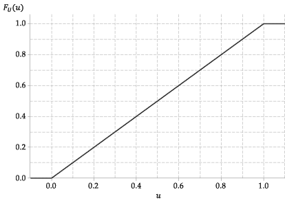
Figure 4: The cumulative distribution function of \(U \stackrel{\mathrm{d}}{=} \mathrm{U}(0,1)\).
You might have noticed a difference in how the interval between 0.3 and 0.4 was treated in the continuous case, compared to the discrete cases. In all of the discrete cases, the upper limits \(0.4, 0.40, 0.400, \dots\) were excluded, while for the continuous random variable it is included. Whenever we are dealing with discrete random variables, whether the inequality is strict or not often matters, and care is needed. For example,
\[ \Pr(0.30 \leq X_2 \leq 0.40) = 11 \times 0.01 = 0.11 \neq 0.1. \]On the other hand, as we noted earlier in this section, for any continuous random variable \(X\), we have \(\Pr(X = x) = 0\). Consequently, for a continuous random variable \(X\) and for \(a \leq b\), we have \(\Pr(X=a) = \Pr(X=b) = 0\) and therefore
\[ \left.\begin{array}{l} \Pr(a < X < b) \\\\ \Pr(a < X \leq b) \\\\ \Pr(a \leq X < b) \\\\ \Pr(a \leq X \leq b) \end{array}\right\} = F_X(b) - F_X(a). \]The cdf is one way to describe the distribution of a continuous random variable. What about the probability function, as used for discrete random variables? As we have just seen, for a continuous random variable, we have \(p_X(x) = \Pr(X = x) = 0\), for all \(x\), so there is no point in using this. In the next section, we look at the appropriate analogue to the probability function for continuous random variables.
Next page - Content - Probability density functions
| This publication is funded by the Australian Government Department of Education, Employment and Workplace Relations |
Contributors Term of use |