Content
Binomial random variables
Define \(X\) to be the number of successes in \(n\) independent Bernoulli trials, each with probability of success \(p\). We now derive the probability function of \(X\). First we note that \(X\) can take the values \(0,1,2,\dots,n\). Hence, there are \(n+1\) possible discrete values for \(X\). We are interested in the probability that \(X\) takes a particular value \(x\). If there are \(x\) successes observed, then there must be \(n-x\) failures observed. One way for this to happen is for the first \(x\) Bernoulli trials to be successes, and the remaining \(n-x\) to be failures. The probability of this is given by \[ \underbrace{p \times p \times \dots \times p}_{x \text{ of these}} \times \underbrace{(1-p) \times (1-p) \times \dots \times (1-p)}_{n-x \text{ of these}} = p^x (1-p)^{n-x}. \]However, this is only one of the many ways that we can obtain \(x\) successes and \(n-x\) failures. They could occur in exactly the opposite order: all \(n-x\) failures first, then \(x\) successes. This outcome, which has the same number of successes as the first outcome but with a different arrangement, also has probability \(p^x (1-p)^{n-x}\). There are many other ways to arrange \(x\) successes and \(n-x\) failures among the \(n\) possible positions. Once we position the \(x\) successes, the positions of the \(n-x\) failures are inevitable.
The number of ways of arranging \(x\) successes in \(n\) trials is equal to the number of ways of choosing \(x\) objects from \(n\) objects, which is equal to \[ \dbinom{n}{x} = \dfrac{n!}{x!(n-x)!} = \dfrac{n \times (n-1) \times (n-2) \times \dots \times (n-x+2) \times (n-x+1)}{x \times (x-1) \times (x-2) \times \dots \times 2 \times 1}. \] (This is discussed in the module The binomial theorem.) Recall that \(0!\) is defined to be 1, and that \(\binom{n}{n} = \binom{n}{0} = 1\). We can now determine the total probability of obtaining \(x\) successes. Each outcome with \(x\) successes and \(n-x\) failures has individual probability \(p^x (1-p)^{n-x}\), and there are \(\binom{n}{x}\) possible arrangements. Hence, the total probability of \(x\) successes in \(n\) independent Bernoulli trials is \[ \dbinom{n}{x}\, p^x (1-p)^{n-x}, \quad \text{for } x = 0,1,2,\dots,n. \]This is the binomial distribution, and it is arguably the most important discrete distribution of all, because of the range of its application.
If \(X\) is the number of successes in \(n\) independent Bernoulli trials, each with probability of success \(p\), then the probability function \(p_X(x)\) of \(X\) is given by \[ p_X(x) = \Pr(X=x) = \dbinom{n}{x}\, p^x (1-p)^{n-x}, \quad \text{for } x = 0,1,2,\dots,n, \] and \(X\) is a binomial random variable with parameters \(n\) and \(p\). We write \(X \stackrel{\mathrm{d}}{=} \mathrm{Bi}(n,p)\). Notes.- The probability of \(n\) successes out of \(n\) trials equals \(\binom{n}{n}\, p^n (1-p)^0 = p^n\), which is the answer we expect from first principles. Similarly, the probability of zero successes out of \(n\) trials is the probability of obtaining \(n\) failures, which is \((1-p)^n\).
- Consider the two essential properties of any probability function \(p_X(x)\):
- \(p_X(x) \geq 0\), for every real number \(x\).
- \(\sum p_X(x) = 1\), where the sum is taken over all values \(x\) for which \(p_X(x) > 0\).
- If we view the formula \[ p_X(x) = \dbinom{n}{x}\, p^x (1-p)^{n-x} \] in isolation, we may wonder whether \(p_X(x) \leq 1\). After all, the number \(\binom{n}{x}\) can be very large: for example, \(\binom{300}{150} \approx 10^{89}\). But in these circumstances, the number \(p^x (1-p)^{n-x}\) is very small: for example, \(0.4^{150}\times 0.6^{150} \approx 10^{-93}\). So it seems that, in the formula for \(p_X(x)\), we may be multiplying a very large number by a very small number. Can we be sure that the product \(p_X(x)\) does not exceed one? The simplest answer is that we know that \(p_X(x) \leq 1\) because we derived \(p_X(x)\) from first principles as a probability. Alternatively, since \(\sum p_X(x) = 1\) and \(p_X(x) \geq 0\), for all possible values of \(X\), it follows that \(p_X(x) \leq 1\).
Example: Multiple-choice test
A teacher sets a short multiple-choice test for her students. The test consists of five questions, each with four choices. For each question, she uses a random number generator to assign the letters A, B, C, D to the choices. So for each question, the chance that any letter corresponds to the correct answer is equal to \(\dfrac{1}{4}\), and the assignments of the letters are independent for different questions. One of her students, Barry, has not studied at all for the test. He decides that he might as well guess 'A' for each question, since there is no penalty for incorrect answers.
Let \(X\) be the number of questions that Barry gets right. His chance of getting a question right is just the chance that the letter 'A' was assigned to the correct answer, which is \(\dfrac{1}{4}\). There are five questions. The outcome for each question can be regarded as 'correct' or 'not correct', and hence as one of two possible outcomes. Each question is independent. We therefore have the structure of a sequence of independent Bernoulli trials, each with probability of success (a correct answer) equal to \(\dfrac{1}{4}\). So \(X\) has a binomial distribution with parameters 5 and \(\dfrac{1}{4}\), that is, \(X \stackrel{\mathrm{d}}{=} \mathrm{Bi}(5,\frac{1}{4})\). The probability function of \(X\) is shown in figure 1.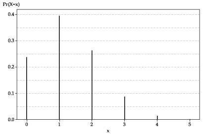
Figure 1: The probability function \(p_X(x)\) for \(X \stackrel{\mathrm{d}}{=} \mathrm{Bi}(5,\frac{1}{4})\).
We can see from the graph that Barry's chance of getting all five questions correct is very small; it is just visible on the graph as a very small value. On the other hand, the chance that he gets none correct (all wrong) is about 0.24, and the chance that he gets one correct is almost 0.4. What are these probabilities, more precisely? The probability function of \(X\) is given by \[ p_X(x) = \dbinom{5}{x}\, \Bigl(\dfrac{1}{4}\Bigr)^x \Bigl(\dfrac{3}{4}\Bigr)^{n-x}, \quad \text{for } x = 0,1,2,3,4,5. \] So \(p_X(5) = \bigl(\dfrac{1}{4}\bigr)^5 \approx 0.0010\); Barry's chance of 'full marks' is one in a thousand. On the other hand, \(p_X(0) = \bigl(\dfrac{3}{4}\bigr)^5 \approx 0.2373\) and \(p_X(1) = 5 \times \dfrac{1}{4} \times \bigl(\dfrac{3}{4}\bigr)^4 \approx 0.3955\). Completing the distribution, we find that \(p_X(2) \approx 0.2637\), \(p_X(3) \approx 0.0879\) and \(p_X(4) \approx 0.0146\).in a cell; this should produce the result 0.2637 (to four decimal places). The somewhat off-putting argument \(\sf \text{FALSE}\) is required to get the actual probability function \(p_X(x)\). If \(\sf \text{TRUE}\) is used instead, then the result is the cumulative probability \(\sum_{k=0}^{x} p_X(k)\), which we do not consider here.
Exercise 1
Casey buys a Venus chocolate bar every day during a promotion that promises 'one in six wrappers is a winner'. Assume that the conditions of the binomial distribution apply: the outcomes for Casey's purchases are independent, and the population of Venus chocolate bars is effectively infinite.
- What is the distribution of the number of winning wrappers in seven days?
- Find the probability that Casey gets no winning wrappers in seven days.
- Casey gets no winning wrappers for the first six days of the week. What is the chance that he will get a winning wrapper on the seventh day?
- Casey buys a bar every day for six weeks. Find the probability that he gets at least three winning wrappers.
- How many days of purchases are required so that Casey's chance of getting at least one winning wrapper is 0.95 or greater?
Exercise 2
Which of the following situations are suitable for modelling with the binomial distribution? For those which are not, explain what the problem is.
- A normal six-sided die is rolled 15 times, and the number of fours obtained is observed.
- For a period of two weeks in a particular city, the number of days on which rain occurs is recorded.
- There are five prizes in a raffle of 100 tickets. Each ticket is either blue, green, yellow or pink, and there are 25 tickets of each colour. The number of blue tickets among the five winning tickets drawn in the raffle is recorded.
- Twenty classes at primary schools are chosen at random, and all the students in these classes are surveyed. The total number of students who like their teacher is recorded.
- Genetic testing is performed on a random sample of 50 Australian women. The number of women in the sample with a gene associated with breast cancer is recorded.
Exercise 3
Ecologists are studying the distributions of plant species in a large forest. They do this by choosing \(n\) quadrats at random (a quadrat is a small rectangular area of land), and examining in detail the species found in each of these quadrats. Suppose that a particular plant species is present in a proportion \(k\) of all possible quadrats, and distributed randomly throughout the forest. How large should the sample size \(n\) be, in order to detect the presence of the species in the forest with probability at least 0.9?
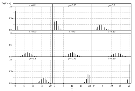
It is useful to get a general picture of the binomial distribution. figure 2 shows nine binomial distributions, each with \(n=20\); the values of \(p\) range from 0.01 to 0.99.
Detailed description
Figure 2: Nine binomial distributions with parameters \(n=20\) and \(p\) as labelled.
A number of features of this figure are worth noting:
- First, we may wonder: Where are all the other probabilities? We know that a binomial random variable can take any value from 0 to \(n\). Here \(n=20\), so there are 21 possible values. But in all of the graphs, there are far fewer than 21 spikes showing. Why? The reason is simply that many of the probabilities are too small to be visible on the scale shown. The smallest visible probabilities are about 0.01; many of the probabilities here are 0.001 or smaller, and therefore invisible. For example (taking an extreme case that is easy to work out), for the top-left graph where \(X \stackrel{\mathrm{d}}{=} \mathrm{Bi}(20,0.01)\), we have \(\Pr(X=20) = 0.01^{20} = 10^{-40}\).
- When \(p\) is close to 0 or 1, the distribution is not symmetric. When \(p\) is close to 0.5, it is closer to being symmetric. When \(p = 0.5\), it is symmetric.
- Consider the pairs of distributions for \(p = \theta\) and \(p = 1-\theta\): \(p = 0.01\) and \(p=0.99\); \(p = 0.05\) and \(p=0.95\); \(p=0.2\) and \(p=0.8\); \(p=0.35\) and \(p=0.65\). Look carefully at the two distributions for any one of these pairs. The two distributions are mirror images, reflected about \(x=10\). This follows from the nature of the binomial distribution.
According to the definition of the binomial distribution, we count the number of successes. Since each of the Bernoulli trials has only two possible outcomes, it must be equivalent, in some sense, to count the number of failures. If we know the number of successes is equal to \(x\), then clearly the number of failures is just \(n-x\). It follows that, if \(X \stackrel{\mathrm{d}}{=} \mathrm{Bi}(n,p)\) and \(Y\) is the number of failures, then \(Y = n-X\) and \(Y \stackrel{\mathrm{d}}{=} \mathrm{Bi}(n,1-p)\). Note that \(X\) and \(Y\) are not independent. - Finally, the spread of the binomial distribution is smaller when \(p\) is close to 0 or 1, and the spread is greatest when \(p = 0.5\).
Next page - Content - Mean and variance
| This publication is funded by the Australian Government Department of Education, Employment and Workplace Relations |
Contributors Term of use |