Content
Variance of a discrete random variable
We have seen that the mean of a random variable \(X\) is a measure of the central location of the distribution of \(X\). If we are summarising features of the distribution of \(X\), it is clear that location is not the only relevant feature. The second most important feature is the spread of the distribution.
If values of \(X\) near its mean \(\mu_X\) are very likely and values further away from \(\mu_X\) have very small probability, then the distribution of \(X\) will be closely concentrated around \(\mu_X\). In this case, the spread of the distribution of \(X\) is small. On the other hand, if values of \(X\) some distance from its mean \(\mu_X\) are likely, the spread of the distribution of \(X\) will be large.
These ideas lead to the most important measure of spread, the variance, and a closely related measure, the standard deviation.
Students have met the concepts of variance and standard deviation when summarising data. These were the sample variance and the sample standard deviation. The difference here is that we are referring to properties of the distribution of a random variable.
The variance of a random variable \(X\) is defined by
\[ \operatorname{var}(X) = \mathrm{E}[(X - \mu)^2], \qquad \text{where \(\mu = \mathrm{E}(X)\).} \]For a discrete random variable \(X\), the variance of \(X\) is obtained as follows:
\[ \operatorname{var}(X) = \sum (x - \mu)^2 p_X(x), \]where the sum is taken over all values of \(x\) for which \(p_X(x) > 0\). So the variance of \(X\) is the weighted average of the squared deviations from the mean \(\mu\), where the weights are given by the probability function \(p_X(x)\) of \(X\).
The standard deviation of \(X\) is defined to be the square root of the variance of \(X\). That is,
\[ \operatorname{sd}(X) = \sigma_X = \sqrt{\operatorname{var}(X)}. \]Because of this definition, the variance of \(X\) is often denoted by \(\sigma_X^2\).
In some ways, the standard deviation is the more tangible of the two measures, since it is in the same units as \(X\). For example, if \(X\) is a random variable measuring lengths in metres, then the standard deviation is in metres (m), while the variance is in square metres (m\(^2\)).
Unlike the mean, there is no simple direct interpretation of the variance or standard deviation. The variance is analogous to the moment of inertia in physics, but that is not necessarily widely understood by students. What is important to understand is that, in relative terms:
- a small standard deviation (or variance) means that the distribution of the random variable is narrowly concentrated around the mean
- a large standard deviation (or variance) means that the distribution is spread out, with some chance of observing values at some distance from the mean.
Note that the variance cannot be negative, because it is an average of squared quantities. This is appropriate, as a negative spread for a distribution does not make sense. Hence, \(\operatorname{var}(X) \geq 0\) and \(\operatorname{sd}(X) \geq 0\) always.
Example
Consider the rolling of a fair six-sided die, with \(X\) the number on the uppermost face. We know that the pf of \(X\) is
\[ p_X(x) = \dfrac{1}{6}, \qquad x=1,2,3,4,5,6, \]and that \(\mu_X = 3.5\). The variance of \(X\) is given by
\begin{align*} \operatorname{var}(X) &= \mathrm{E}[(X - \mu_X)^2] \\ &= \sum (x - \mu_X)^2 p_X(x) \\ &= \sum (x - \mu_X)^2 \dfrac{1}{6} \\ &= \dfrac{1}{6} \Bigl( (1-3.5)^2 + (2-3.5)^2 + (3-3.5)^2 + (4-3.5)^2 + (5-3.5)^2 + (6-3.5)^2 \Bigr)\\ &= \dfrac{1}{6} \times 17.5 \\ &= \dfrac{35}{12} \approx 2.9167. \end{align*}Hence, the standard deviation of \(X\) is \(\sigma_X = \sqrt{\dfrac{35}{12}} \approx 1.7078\).
Exercise 7
Consider again the example of the number of languages spoken by Australian school children. Define \(X\) to be the number of languages in which a randomly chosen Australian child attending school can hold an everyday conversation. Assume that the probability function of \(X\), \(p_X(x)\), is as shown in the following table.
| \(x\) | 1 | 2 | 3 | 4 | 5 | 6 |
|---|---|---|---|---|---|---|
| \(p_X(x)\) | 0.663 | 0.226 | 0.066 | 0.022 | 0.019 | 0.004 |
- What is the mean of \(X\)?
- Find the variance and standard deviation of \(X\).
- What are the units of the mean and standard deviation?
Exercise 8
Consider the following four discrete distributions.
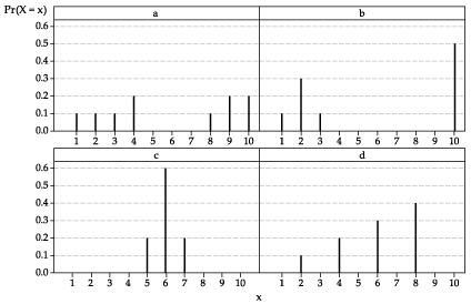
- Confirm that each graph represents a probability function.
- Guess the value of the mean of each corresponding random variable.
- Calculate the value of the mean in each case.
- Guess the order of the variances, from largest to smallest.
- Find the variance and standard deviation in each case.
Next page - Answers to exercises
| This publication is funded by the Australian Government Department of Education, Employment and Workplace Relations |
Contributors Term of use |