Content
Mean of a discrete random variable
If you roll a fair die many times, what will be the average outcome? Imagine rolling it 6000 times. You would expect to roll about 1000 ones, 1000 twos, and so on: about 1000 occurrences of each possible outcome. What would be the average value of the outcomes obtained? Approximately, the average or mean would be
\[ \dfrac {(1000 \times 1) + (1000 \times 2) + \dots + (1000 \times 6)} {6000} = \dfrac{21\ 000}{6000} = 3.5. \]This can be thought of as the weighted average of the six possible values \(1,2,\dots,6\), with weights given by the relative frequencies. Note that 3.5 is not a value that we can actually observe.
By analogy with data and relative frequencies, we can define the mean of a discrete random variable using probabilities from its distribution, as follows.
The mean \(\mu_X\) of a discrete random variable \(X\) with probability function \(p_X(x)\) is given by
\[ \mu_X = \sum x\, p_X(x), \]where the sum is taken over all values \(x\) for which \(p_X(x) > 0\).
The mean can be regarded as a measure of `central location' of a random variable. It is the weighted average of the values that \(X\) can take, with weights provided by the probability distribution.
The mean is also sometimes called the expected value or expectation of \(X\) and denoted by \(\mathrm{E}(X)\). These are both somewhat curious terms to use; it is important to understand that they refer to the long-run average. The mean is the value that we expect the long-run average to approach. It is not the value of \(X\) that we expect to observe.
Consider a random variable \(U\) that has the discrete uniform distribution with possible values \(1,2,\dots,m\). The mean is given by
\begin{align*} \mu_U &= \sum_{x=1}^{m} \Bigl(x \times \dfrac{1}{m}\Bigr) \\\\ &= \dfrac{1}{m}\, \sum_{x=1}^m x \\\\ &= \dfrac{1}{m} \times \dfrac{m(m+1)}{2} \\\\ &= \dfrac{m+1}{2}. \end{align*}For example, the mean for the roll of a fair die is \(\dfrac{6 + 1}{2} = 3.5\), as expected.
So in the long run, rolling a single die many times and obtaining the average of all the outcomes, we `expect' the average to be close to 3.5, and the more rolls we carry out, the closer the average will be.
The use of the terms `expected value' and `expectation' is the reason for the notation \(\mathrm{E}(X)\), which also extends to functions of \(X\).
Exercise 4
Consider again the biased die made by Sneaky Sam. Recall that the distribution of \(X\), the number of spots on the uppermost face when the die is rolled, is as follows.
| \(x\) | 1 | 2 | 3 | 4 | 5 | 6 |
|---|---|---|---|---|---|---|
| \(p_X(x)\) | \(\dfrac{1-\theta}{6}\) | \(\dfrac{1-\theta}{6}\) | \(\dfrac{1-\theta}{6}\) | \(\dfrac{1+\theta}{6}\) | \(\dfrac{1+\theta}{6}\) | \(\dfrac{1+\theta}{6}\) |
- Find \(\mu_X\), the mean of \(X\).
- What is the largest possible value of \(\mu_X\)?
The following graph shows once again the probability function for the outcome of rolling a fair die. This distribution is symmetric, and the mean 3.5 is in the middle of the distribution; in fact, it is on the axis of symmetry.
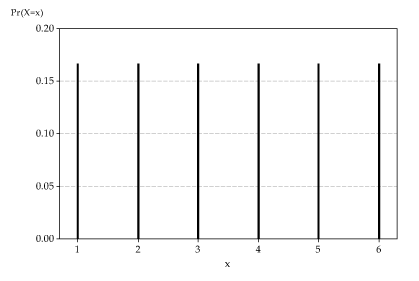
Detailed description
The distribution of \(X\), the number on the uppermost face when a fair die is rolled.
We can give a general physical interpretation of the mean of a discrete random variable \(X\) with pf \(p_X(x)\). Suppose we imagine that the \(x\)-axis is an infinite see-saw in each direction, and we place weights equal to \(p_X(x)\) at each possible value \(x\) of \(X\). Then the mean \(\mu_X\) is at the point which will make the see-saw balance. In other words, it is at the centre of mass of the system.
If the distribution of a discrete random variable is represented graphically, then you should be able to guess the value of its mean, at least approximately, by using the `centre of mass' idea. This is the topic of the next exercise.
Exercise 5
The distributions (labelled 'a' to 'f') of six different random variables are shown below.
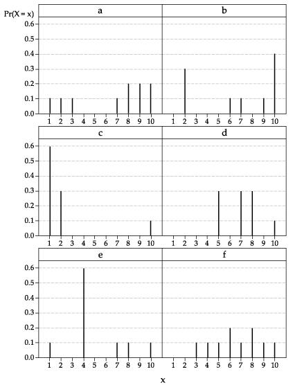
For each distribution separately:
- Confirm that the graph represents a probability function.
- Guess the value of the mean of the corresponding random variable.
- Calculate the value of the mean.
Suppose that \(X\) has a geometric distribution with parameter \(p\), and therefore its probability function is
\[ p_X(x) = p (1-p)^x, \qquad x=0,1,2,\dots. \]Recall that \(X\) is the number of trials before the first success in a sequence of independent trials, each with probability of success \(p\). Do you expect there to be many trials before the first success, on average, or just a few?
A result which we state here without proof is that, for \(X \stackrel{\mathrm{d}}{=} G(p)\), we have
\[ \mu_X = \dfrac{1-p}{p}. \]If \(p\) is large (that is, close to 1), then successes are very likely and the wait before the first success is likely to be short; in this case, \(\mu_X\) is small. On the other hand, if \(p\) is small (close to 0), then failures are very likely and the wait before the first success is likely to be long; in this case, \(\mu_X\) is large.
Exercise 6
- One of the standard forms of commercial lottery selects six balls at random out of 45. What is the chance of winning first prize in such a lottery with a single entry?
- Suppose that someone buys a single entry in every draw. What is the distribution of the number of draws entered before the player wins first prize for the first time?
- What is the expected number of draws before winning first prize for the first time?
- Suppose the draws occur weekly. On average, how many years does the person have to wait before winning first prize for the first time?
We may wish to find the mean of a function of a random variable \(X\), such as \(X^2\) or \(\log X\). For a discrete random variable \(X\) with pf \(p_X(x)\), consider an arbitrary function of \(X\), say \(Y = g(X)\). Then the expectation of \(Y\), that is, \(\mathrm{E}(Y) = \mu_Y\), is obtained as follows:
\begin{alignat*}{2} \mu_Y &= \sum y\, \Pr(Y=y) &\qquad&\text{(summing over \(y\) for which \(\Pr(Y=y) > 0\))} \\\\ &= \sum g(x)\, \Pr(X=x) & &\text{(summing over \(x\) for which \(\Pr(X=x) > 0\))} \\\\ &= \sum g(x)\, p_X(x). \end{alignat*}For the special case of a linear transformation \(Y = aX + b\), we shall see that it follows that \(\mu_Y = a \mu_X + b\). This is a very useful result; it says that, for a linear transformation, the mean of the transformed variable equals the transformation of the mean of the original variable. In particular, if \(Y = aX\), then \(\mu_Y = a\mu_X\), as you might expect. This applies to changes of units: for example, if the random variable \(X\) measures a time interval in days, and we wish to consider the equivalent time in hours, then we can define \(Y = 24X\) and we know that \(\mu_Y = 24\mu_X\).
For a transformation \(Y = g(X)\), it is not true in general that \(\mu_Y = g(\mu_X)\). But in the special case of a linear transformation \(Y = aX + b\), where \(g(x) = ax + b\), we have
\begin{align*} \mu_Y &= \sum g(x)\, p_X(x) \\\\ &= \sum (ax + b)\, p_X(x) \\\\ &= \sum ax\, p_X(x) + \sum b\, p_X(x) \\\\ &= a \sum x\, p_X(x) + b \sum p_X(x) \\\\ &= a\mu_X + b, \end{align*}as claimed.
Technical note. Every discrete random variable \(X\) with a finite set of possible values has a mean \(\mu_X\). But it is possible to construct examples where the mean does not exist. For example, consider the discrete random variable \(X\) with probability function \(p_X(x) = \dfrac{1}{x}\), for \(x = 2,4,8,16,\dots\). Here \(\sum p_X(x) = \sum_{n=1}^\infty \dfrac{1}{2^n} = 1\), as required for a probability function. But \(\mu_X = \sum x\, p_X(x) = \sum_{n=1}^\infty 1\) does not exist. Such complications are not considered in secondary school mathematics.Next page - Content - Variance of a discrete random variable
| This publication is funded by the Australian Government Department of Education, Employment and Workplace Relations |
Contributors Term of use |