Content
Examples of discrete distributions
Discrete uniform distribution
In the previous two sections, we considered the random variable defined as the number on the uppermost face when a fair die is rolled. This is an example of a random variable with a discrete uniform distribution. In general, for a positive integer \(m\), let \(X\) be a discrete random variable with pf \(p_X(x)\) given by
\[ p_X(x) = \Pr(X = x) = \begin{cases}^\frac{1}{m} &\text{if \(x=1,2,\dots,m\),} \\ 0 &\text{otherwise.} \end{cases} \]Then \(X\) has a discrete uniform distribution. This is a distribution that arises often in lotteries and games of chance.
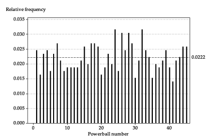
We have seen this distribution in the Powerball example considered in the module Probability. In commercial lotteries, such as Powerball, it is a regulatory requirement that each outcome is equally likely. There are 45 possible Powerball numbers (\(1,2,\dots,45\)). So if \(X\) is the Powerball drawn on a particular occasion, the pf \(p_X(x)\) of \(X\) is given by
\[ p_X(x) = \Pr(X = x) = \begin{cases}^\frac{1}{45} &\text{if \(x=1,2,\dots,45\),} \\ 0 &\text{otherwise.} \end{cases} \]If this model for the drawing of Powerball numbers is correct, we should expect that, over a large number of draws, the relative frequencies of the 45 possible numbers are all approximately equal to \(\tfrac{1}{45} \approx 0.0222\). The following graph shows the relative frequencies observed in the 853 draws from May 1996 to September 2012.
Detailed description
Relative frequencies of Powerball numbers over 853 draws.
The model probability of 0.0222 is shown as a reference line.
Geometric distribution
The set of possible values for a discrete random variable may be infinite, as the following example shows.
Example
Fix a real number \(p\) with \(0 < p < 1\). Now let \(X\) be the discrete random variable with probability function \(p_X(x)\) given by
\[ p_X(x) = \Pr(X = x) = \begin{cases} p(1-p)^x &\text{if \(x=0,1,2,\dots\),} \\ 0 &\text{otherwise.} \end{cases} \]We will confirm that \(p_X(x)\) has the two requisite properties of a probability function. First, we have \(p_X(x) \geq 0\), since \(p > 0\) and \(1-p > 0\). Second, we have
\begin{alignat*}{2} \sum p_X(x) &= p + p(1-p) + p(1-p)^2 + \dotsb \\\\ &= p\, \bigl(1 + (1-p) + (1-p)^2 + \dotsb \bigr) \\\\ &= p\, \Bigl(\dfrac{1}{1 - (1-p)}\Bigr) &\qquad &\text{(sum of an infinite geometric series)} \\\\ &= 1. \end{alignat*}Suppose that a sequence of independent `trials' occur, and at each trial the probability of `success' equals \(p\). Define \(X\) to be the number of trials that occur before the first success is observed. Then \(X\) has a geometric distribution with parameter \(p\).
We introduce here a symbol used throughout the modules on probability and statistics. If \(X\) has a geometric distribution with parameter \(p\), we write \(X \stackrel{\mathrm{d}}{=} G(p)\). The symbol \(\stackrel{\mathrm{d}}{=}\) stands for `has the distribution', meaning the distribution indicated immediately to the right of the symbol.
Note the use of the generic terms `trial' and `success'. They are arbitrary, but they carry with them the idea of each observation involving a kind of test (i.e., trial) in which we ask the question: Which one of the two possibilities will be observed, a `success' or a `failure'? In this sense, the words `success' and `failure' are just labels to keep track of the two possibilities for each trial.
Note that \(X\) can take the value 0, if a success is observed at the very first trial. Or it can take the value 1, if a failure is observed at the first trial and then a success at the second trial. And so on. What is the largest value that \(X\) can take? There is no upper limit, in theory. As the values of \(X\) increase, the probabilities become smaller and smaller. The sum of the probabilities equals one, as shown in the previous example.
Exercise 2
Recall that Tetris pieces have seven possible shapes, labelled \(\mathtt{I}, \mathtt{J}, \mathtt{L}, \mathtt{O}, \mathtt{S}, \mathtt{T}, \mathtt{Z}\). Assume that, at any stage of the game, all seven shapes are equally likely to be produced, independent of whatever pieces have been produced previously.
Consider the sequences of three consecutive pieces observed during a game of Tetris, such as \(\mathtt{JLL}\), \(\mathtt{ZOS}\), \(\mathtt{ZSZ}\), \(\mathtt{III}\) and so on.
- What is the probability that a sequence of three pieces does not contain a \(\mathtt{Z}\)?
- Hence, what is the probability that a sequence of three pieces has at least one \(\mathtt{Z}\)?
- What is the probability that a \(\mathtt{Z}\) occurs in the first three-piece sequence observed?
- What is the probability that a \(\mathtt{Z}\) does not occur in the first three-piece sequence, but does occur in the second such sequence? (Here we are considering non-overlapping sequences of three pieces.)
- What is the probability that a \(\mathtt{Z}\) does not occur in the first \(x\) three-piece sequences, but does occur in the \((x+1)\)st such sequence?
- Hence, what is the distribution of \(X\), the number of three-piece sequences observed before a three-piece sequence with a \(\mathtt{Z}\) in it first appears? Write down its probability function \(p_X(x)\).
- Evaluate \(p_X(x)\) for \(x = 2,3,4,10\).
Exercise 3
Julia and Tony play the hand game Rock-paper-scissors. Assume that, at each play, they make their choices with equal probability (\(\tfrac{1}{3}\)) for each of the three moves, independently of any previous play.
- On any single play, what is the chance of a tie?
- What is the chance that Julia wins at the first play?
- Define \(X\) to be the number of plays before Julia wins for the first time. What is the distribution of \(X\)?
- Write down the probability function \(p_X(x)\) of \(X\).
- Find \(\Pr(X = 5)\).
- Find \(\Pr(X \geq 5)\).
Another important distribution arises in the context of a sequence of independent trials that each have the same probability of success \(p\). This is the binomial distribution. There is an entire module devoted to it (Binomial distribution), so we do not consider it further here.
Next page - Content - Mean of a discrete random variable
| This publication is funded by the Australian Government Department of Education, Employment and Workplace Relations |
Contributors Term of use |