Content
Probability functions
To work out the probability that a discrete random variable \(X\) takes a particular value \(x\), we need to identify the event (the set of possible outcomes) that corresponds to "\(X = x\)".
In general, the function used to describe the probability distribution of a discrete random variable is called its probability function (abbreviated as pf). The probability function of \(X\) is the function \(p_X \colon \mathbb{R} \to [0,1]\) given by
\[ p_X(x) = \Pr(X=x). \]In general, the probability function \(p_X(x)\) may be specified in a variety of ways. One way is to specify a numerical value for each possible value of \(X\); we have done that for the die-rolling example. In the die-rolling example, the random variable \(X\) can take exactly six values, and no others, and we assert that the probability that \(X\) takes any one of these values is the same, namely \(\dfrac{1}{6}\).
As is the case generally for functions, the lower-case \(x\) here is merely the argument of the function. If we write \(\Pr(X = y)\) it is essentially the same function, just as \(f(x) = 2x^2 + 3x - 1\) and \(f(y) = 2y^2 + 3y - 1\) are the same function. But it helps to associate the corresponding lower-case letter with the random variable we are considering.
Another way to specify the probability function is using a formula. We will see examples of this in the next section.
Less formally, the probability distribution may be represented using a graph, with a spike of height \(p_X(x)\) at each possible value \(x\) of \(X\). If there are too many possible values of \(X\) for this visual representation to work, we may choose to omit probabilities that are very close to zero; such values will typically be invisible on a graph anyway.
The following graph shows the probability function for the outcome of rolling a fair die.
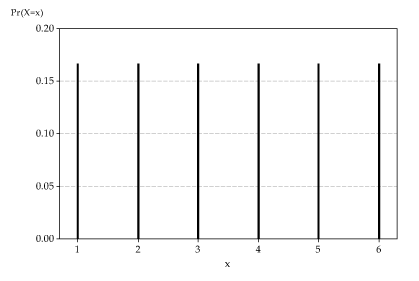
Detailed description
The distribution of \(X\), the number on the uppermost face when a fair die is rolled.
The importance of the notational convention to use capital letters for random variables now becomes apparent. A random variable \(X\) has a distribution. Formally, \(X\) is a function from the event space to the real line. An observed value of \(X\), such as \(x=4\), is simply a number. Once we have rolled the die, we have the outcome. If we observed \(x=4\), this does not have a distribution. It is the observed value, and a number.
Quite often, there is more than one random variable being considered. That is the reason for writing \(p_X(x)\) for the probability function of \(X\), to distinguish it from \(p_Y(y)\), say, the probability function of \(Y\).
Since the probability function \(p_X(x)\) is a probability, it must obey the axioms. Two important properties of a probability function follow from this:
- \(p_X(x) = \Pr(X = x) \geq 0\), for every real number \(x\).
- \(\sum p_X(x) = 1\), where the sum is taken over all values \(x\) for which \(p_X(x) > 0\).
In fact, these two properties characterise probability functions. If a function \(f \colon \mathbb{R} \to \mathbb{R}\) satisfies these two properties, then we can view \(f\) as the probability function of a discrete random variable.
Exercise 1
Sneaky Sam has manufactured a deliberately biased six-sided die, with the following probability distribution for \(X\), the number of spots on the uppermost face when the die is rolled.
| \(x\) | 1 | 2 | 3 | 4 | 5 | 6 |
|---|---|---|---|---|---|---|
| \(p_X(x)\) | \(\dfrac{1-\theta}{6}\) | \(\dfrac{1-\theta}{6}\) | \(\dfrac{1-\theta}{6}\) | \(\dfrac{1+\theta}{6}\) | \(\dfrac{1+\theta}{6}\) | \(\dfrac{1+\theta}{6}\) |
- What values of \(\theta\) are feasible, in order for \(p_X(x)\) to be a probability function?
- Find \(\Pr(X \geq 4)\) in terms of \(\theta\).
- Find \(\Pr(3 \leq X \leq 4)\).
- What is the probability of rolling an even number?
Random variables arising in practical settings of real importance are often much less readily dealt with than those arising in dice rolling. A common approach in such situations, which directly mirrors one of the approaches to probability, is to estimate the probability distribution of the random variable from data.
Example
Consider the random variable \(X\) defined to be the number of languages in which a randomly chosen Australian child attending school can hold an everyday conversation. Suppose we take a random sample of 1000 Australian school children and obtain the following data for the number of languages spoken.
| \(x\) | 1 | 2 | 3 | 4 | 5 | 6 | Total |
|---|---|---|---|---|---|---|---|
| Frequency | 663 | 226 | 66 | 22 | 19 | 4 | 1000 |
Then we obtain an estimate of \(p_X(x)\), the pf of \(X\), from the relative frequencies.
| \(x\) | 1 | 2 | 3 | 4 | 5 | 6 |
|---|---|---|---|---|---|---|
| Estimate of \(p_X(x)\) | 0.663 | 0.226 | 0.066 | 0.022 | 0.019 | 0.004 |
So we estimate that \(22.6\%\) of Australian school children can hold an everyday conversation in (exactly) two languages; equivalently, we estimate that \(\Pr(X=2) = 0.226\).
In this case, we cannot be sure that \(x=7\) (for example) is an impossible value. It may just be so rare that it did not crop up in the sample.
Next page - Content - Examples of discrete distributions
| This publication is funded by the Australian Government Department of Education, Employment and Workplace Relations |
Contributors Term of use |