Answers to exercises
Exercise 1
The first stage of mixing ensures that the first ball is sampled at random. We can think of it as a random sample of size \(n=1\). In fact, any subsequent re-mixing is redundant. As the initial mixing ensures the first ball is randomly sampled, any subsequent balls sampled without additional mixing will also be randomly sampled. If this were not the case, the choice of the first ball could not be considered random. So the subsequent mixing is presumably done to reassure psychologically those playing the game, rather than for reasons of randomness.
Exercise 2
- There are only two possible samples that can be chosen. Note that if a simple random sample of \(n=150\) is chosen from a population of size \(N = 300\), the number of possible samples is huge: approximately \(10^{89}\).
- Yes, each student has probability 0.5 of being selected.
- This is not a simple random sample, because the process does not give every possible sample of size \(n=150\) the same chance of being selected.
Exercise 3
- The electoral roll would be imperfect as a sample frame. For example, young people who were eligible voters but had not yet registered to vote would not be included. The extent of this potential bias might, for example, depend on the recency of an election.
- If 60 000 people were summoned from 3.5 million voters in Victoria, the probability of selection in one year is \(\dfrac{60\ 000}{3\ 500\ 000} \approx 0.017\), or \(1.7\%\).
- There are a number of things we need to know to determine if an individual could be called up for jury duty twice in one year. If the random sample of potential jurors for a given year is taken at a single point in time, using a method like that described using Excel, then each individual will have only one chance of selection. If the sample is taken across the year, the potential to be sampled twice will depend on whether or not an individual is exempt once they have been sampled. In fact, individuals in metropolitan Melbourne who attend for jury service but do not serve as a juror on a trial are excluded from the sample frame for two years.
- If you only had access to a hard copy of the electoral roll, organised by electorate, the sampling would need to be done in stages. You might, for example, first select a subset of electorates; you could take a simple random sample of electorates. Next you would need to consider practical ways to sample from the book listing names in each electorate. You could, for example, find the number of pages in a selected book and take a random sample of pages. You might consider summoning all the people listed on a sampled page; this is a kind of cluster sampling. However, this is unlikely to be ideal: electoral rolls are organised alphabetically and so people on the same page are likely to be related. It would be better to randomly sample some individuals from a selected page. If random sampling is used at every stage, the resulting sample is a random sample. It would not be a simple random sample if, for example, the same number of people were sampled from each selected electorate; people in smaller electorates would have a greater chance of selection than people in larger electorates.
Exercise 4
- The question the survey asks is quite provocative, and people might respond for a range of reasons. All will be self-selected volunteers. Some people might simply be motivated to engage with the survey because of the provoking title. Others may have strong views about prescription-drug use and want to make sure they are counted. The survey states that it is 'girls only', but there are no restrictions on who can enter the responses online. Sometimes prizes or monetary rewards are offered for participating in surveys; this can motivate participants, but was not the case for the Cosmopolitan survey.
- We have no idea who has provided the answers to the questions asked in this online survey. It is open to the usual biases of self-selected samples, but also to the whims of mischievous internet users. There is no quality control, leaving great potential for bias. The actual bias is unknown, so we learn nothing, or very little, about the population of interest.
Exercise 5
- One obvious strategy would be to access boys aged 13 to 16 through schools. The minimum school leaving age is 17, but there are options to participate in approved school-equivalent programs for 15- and 16-year-olds. Participants in these alternative programs would not be accessed through schools, and so ways of identifying and sampling boys in this group would need to be developed. This might be able to be done via registrations of participants in the approved school-equivalent programs. Sampling in stages would be needed; for example, schools and then classes might be sampled. It would be efficient to sample all boys within a given class.
- Following these adolescents over time may become difficult as they leave school, leave home and transition into adult life.
- It may be that the boys/men who are most difficult to track over time are those with problematic drug and alcohol use.
- The purpose of the study is look at the effects of drug and alcohol use; if the heavier users are more difficult to track and less likely to be able to be followed up, the effects may be underestimated.
Exercise 6
- Over 27000 respondents sounds impressive, but if the sample is badly biased, a large sample size does not guarantee validity: think of the Literary Digest poll.
The Age poll was an online poll accessible by computer users. Some sectors of the community would not be able to access the poll.
 - People with an interest in the election outcome are likely to respond to this kind of poll. It is possible to vote more than once in such polls, and this may have happened.
- The disclaimer indicated that the poll was not scientific; The Age polls often have a disclaimer indicating that the poll is based on views of volunteers. However, despite the caveat, The Age suggested that the results will concern Labor supporters.
Exercise 7
- If the poll was unbiased, the percentage vote predicted for Roosevelt is the observed proportion in the poll: 43%.
- Among the \(2\ 400\ 000\) respondents, there are \(2\ 400\ 000 \times 0.43 = 1\ 032\ 000\) votes for Roosevelt. If all \(7\ 600\ 000\) non-respondents vote for Roosevelt, then the total number of votes for him is \(1\ 032\ 000 + 7\ 600\ 000 = 8\ 632\ 000\) out of \(10\ 000\ 000\). Hence the predicted percentage vote for Roosevelt is 86%.
- From the \(2\ 400\ 000\) respondents, there are \(1\ 032\ 000\) votes for Roosevelt. If all of the \(7\ 600\ 000\) non-respondents vote for Landon, the total number of votes for Roosevelt is \(1\ 032\ 000 + 0 = 1\ 032\ 000\) out of \(10\ 000\ 000\). Hence the predicted percentage vote for Roosevelt is 10%.
- From the \(2\ 400\ 000\) respondents, there are \(1\ 032\ 000\) votes for Roosevelt. If half of the \(7\ 600\ 000\) non-respondents vote for Roosevelt, then the total number of votes for him is \(1\ 032\ 000 + 3\ 800\ 000 = 4\ 832\ 000\) out of \(10\ 000\ 000\). Hence the predicted percentage vote for Roosevelt is 48%.
- To obtain 62% of the vote from the \(10\ 000\ 000\) people sampled, Roosevelt would need \(6\ 200\ 000\) votes. From the \(2\ 400\ 000\) respondents, he received \(1\ 032\ 000\) votes; hence, he would need to receive \(6\ 200\ 000 - 1\ 032\ 000 = 5\ 168\ 000\) votes from the \(7\ 600\ 000\) non-respondents. This is \(\dfrac{5\ 168\ 000}{7\ 600\ 000} = 0.68\), or 68%, of the non-respondents' vote. Contrast this with the 43% he received from the respondents.
Exercise 8
- Let \(X \stackrel{\mathrm{d}}{=} \mathrm{N}(30, 7^2)\). Then \(\Pr(X < 30) = \dfrac{1}{2}\), because the Normal distribution is symmetric and its mean and median are equal. In a random sample, all observations are independent, so the probability than all 10 observations are below 30 is equal to the product of the individual probabilities, and is therefore equal to \((\dfrac{1}{2})^{10} \approx 0.001\).
- 0.001, by symmetry.
- 0.002; the two events are mutually exclusive, so we can add the two probabilities.
- No. About one in every 500 samples (actually, one in every 512) will have this feature, so it is not surprising that we have observed 100 samples and none of them has the feature.
- It is not that easy to tell this, just from inspection of the dotplots. The largest mean is 34.7, for the sample in row 2, column 6. The smallest mean is 24.1, for the sample in row 4, column 9.
- \(\Pr(X \leq 16) = \Phi(-2) \approx 0.0228\).
- \(Y \stackrel{\mathrm{d}}{=} \mathrm{Bi}(10,0.0228)\).
- \(\Pr(Y \geq 3) \approx 0.0013\). This is indeed quite an unusual sample.
- If we regard an observation of \(y = 3\) as unusual, we must regard \(y \geq 4\) as even more unusual, so we count more extreme values in the calculation. Think of a very hot day in summer; suppose the maximum reached is 44.3 \(^\circ\)C. If we wonder how extreme this is, we do not ask: 'How common are days with a maximum of 44.3 \(^\circ\)C?' Rather, we ask: 'How common are days with a maximum of at least 44.3 \(^\circ\)C?'
Exercise 9
Figure 33 provides the missing pdfs. You may not get the answers exactly right, based only on a visual impression. But you should be able to get within about 1 of the correct value of each mean and standard deviation, just by eye. This is a preliminary to the more formal approaches of inference, which is dealt with in the two modules Inference for proportions and Inference for means.
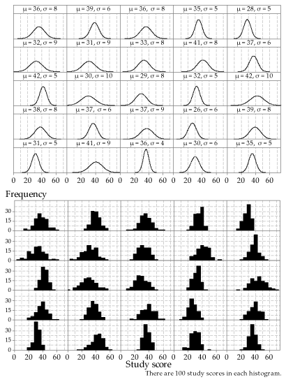
Figure 33: 25 different Normal distributions (upper part) and histograms of random samples from each of them (lower part); the same sample size \(n=100\) has been used throughout.
| This publication is funded by the Australian Government Department of Education, Employment and Workplace Relations |
Contributors Term of use |