Content

Sampling from the binomial distribution

In the module Binomial distribution, we saw that from a random sample of \(n\) observations on a Bernoulli random variable, the sum of the observations \(X\) has a binomial distribution. We revisit this theory briefly.

A Bernoulli random variable is a simple discrete random variable that takes the value 1 with probability \(p\) and the value 0 with probability \(1-p\). This is a suitable distribution to model sampling from an essentially infinite population of units in which a proportion \(p\) of the units have a particular characteristic. If we choose a unit at random from this population, the probability that it has the characteristic is equal to \(p\), and the probability that it does not have the characteristic is equal to \(1-p\).

We may label the presence of the characteristic as '1' and its absence as '0'. So we consider \(Y \stackrel{\mathrm{d}}{=} \mathrm{Bernoulli}(p)\), which satisfies \(\Pr(Y = 1) = p\) and \(\Pr(Y = 0) = 1-p\).

We take a random sample \(Y_1,Y_2,\dots,Y_n\) from this distribution. This means that these random variables are independent and identically distributed, with \(Y_i \stackrel{\mathrm{d}}{=} \mathrm{Bernoulli}(p)\), for \(i=1,2,\dots,n\).

Define \(X = \sum_{i=1}^{n} Y_i\); then \(X \stackrel{\mathrm{d}}{=} \mathrm{Bi}(n,p)\). The sum of the \(Y_i\)'s is equal to the number of units in the sample with the characteristic of interest.

Suppose we obtain a random sample from a population of voters in Australia in which the proportion that support the Australian Labor Party is \(p=0.5\). We use this context to explore the binomial distribution. (In fact, in federal elections in Australia, the two-party-preferred vote is often quite close to 50%, corresponding to \(p=0.5\). For example, in the 2010 federal election, the two-party-preferred vote for Labor was \(50.1\%\).) The population of voters in Australia is large enough to be regarded as effectively infinite for the purposes of this discussion.

Unlike the cases considered so far, note that each of the random samples gives a single observation from the \(\mathrm{Bi}(n,p)\) distribution (rather than many). In each case it is based on a random sample of size \(n\) from the Bernoulli distribution.

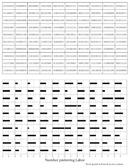
Consider figure 28. It represents 100 distinct observation on the \(\mathrm{Bi}(10,0.5)\) distribution, coming from 100 random samples each of size \(n=10\) from the \(\mathrm{Bernoulli}(0.5)\) distribution. The details of the 10 observations in each random sample are shown by the individual zeroes and ones listed. For example, in the top left-hand sample, there are 5 ones, giving an observation \(x=5\) from the \(\mathrm{Bi}(10,0.5)\) distribution. This observation is represented by the bar of length 5 in the top left-hand panel of the lower part of the figure.

Detailed description

Figure 28: 100 random samples of size \(n=10\) from the \(\mathrm{Bernoulli}(0.5)\) distribution (upper part) giving 100 corresponding observations from the \(\mathrm{Bi}(10,0.5)\) distribution (lower part).

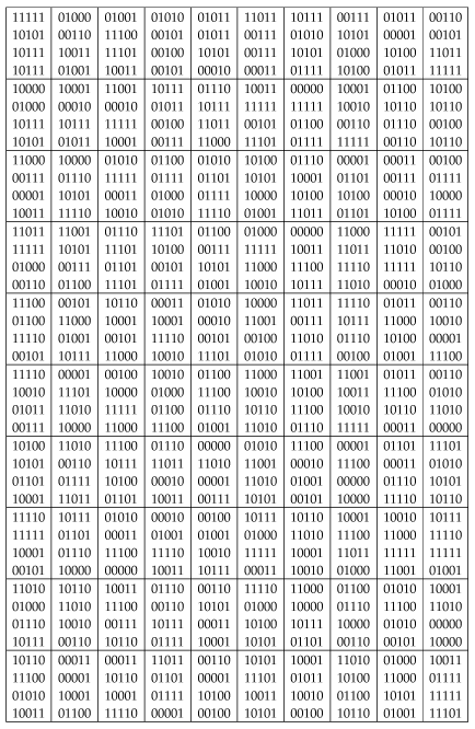
Figure 29 lists 100 random samples of size \(n=20\) from the \(\mathrm{Bernoulli}(0.5)\) distribution. Of course, as the sample size increases, it starts to get tedious to list all those zeroes and ones! And we don't need to: given the assumptions, the information of interest is really just the total number of ones in the sample, which is exactly what is measured by the binomial random variable.

Detailed description

Figure 29: 100 random samples of size \(n=20\) from the \(\mathrm{Bernoulli}(0.5)\) distribution.

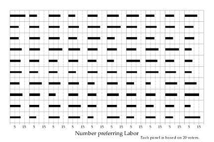
The binomial observations from the Bernoulli random samples of size \(n=20\) listed in figure 29 are shown in figure 30.

Detailed description

Figure 30: 100 observations from the \(\mathrm{Bi}(20,0.5)\) distribution arising from the Bernoulli random samples in figure 29.

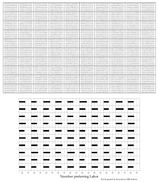
Now we represent samples from the binomial distribution with \(n=100\) and \(p=0.5\).

Detailed description

Figure 31: 100 random samples of size \(n=100\) from the \(\mathrm{Bernoulli}(0.5)\) distribution (upper part) giving 100 corresponding observations from the \(\mathrm{Bi}(100,0.5)\) distribution (lower part).

Finally, we look at what happens when we vary the value of \(p\). Figure 32 shows independent observations from the \(\mathrm{Bi}(40,p)\) distribution for \(p = 0.1,0.2,\dots,0.9\). Ten observations are shown for each value of \(p\). Note how \(p\) influences the values obtained. For \(p=0.1\) (the lowest value shown), the number observed in all 10 cases was less than 10. For \(p = 0.9\), all 10 observations were over 30. For \(p=0.5\), the observations were near 20.

Detailed description

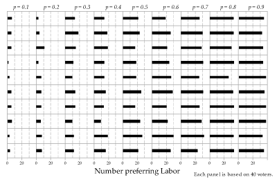
Figure 32: Observations from the \(\mathrm{Bi}(40,p)\) distribution; the value of \(p\) is constant for each column.

Next page - Answers to exercises