Content
Sampling from the continuous uniform distribution
Now we consider samples from the continuous uniform distribution.
Recall from the module Continuous probability distributions that, if the random variable \(U\) has a uniform distribution on the interval \((a, b)\), which we write as \(U \stackrel{\mathrm{d}}{=} \mathrm{U}(a,b)\), then \(U\) has the following pdf:
\[ f_U(u) = \begin{cases} \dfrac{1}{b-a} & \text{if \(a < u < b\),}\\ 0 &\text{otherwise.} \end{cases} \]In particular, if \(U \stackrel{\mathrm{d}}{=} \mathrm{U}(0,1)\), then
\[ f_U(u) = \begin{cases} 1 &\text{if \(0 < u < 1\),}\\ 0 &\text{otherwise.} \end{cases} \]We saw this distribution in the section Mechanisms for generating random samples, where we discussed obtaining a random sample in Excel. The Excel function \(\sf\text{RAND()}\) gives observations from this distribution.
Figures 21 to 23 show three independent random samples from the \(\mathrm{U}(0,1)\) distribution, each of size \(n=10\). Note how they vary.
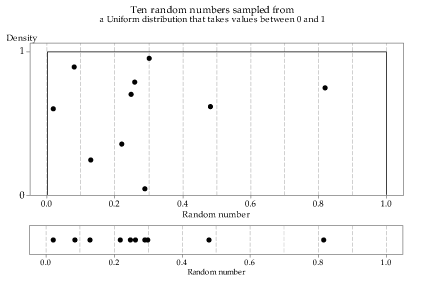
Figure 21: First random sample of size \(n=10\) from the \(\mathrm{U}(0,1)\) distribution.
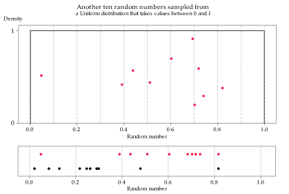
Figure 22: Second random sample of size \(n=10\) from the \(\mathrm{U}(0,1)\) distribution.
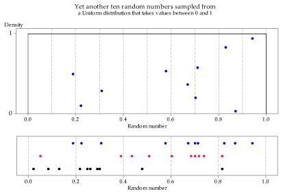
Figure 23: Third random sample of size \(n=10\) from the \(\mathrm{U}(0,1)\) distribution.
Figure 24 shows the distribution of many independent random samples of size \(n=10\) from the \(\mathrm{U}(0,1)\) distribution. Remember that this means that any single observation in any of the samples is equally likely to be observed at any point along the number line between 0 and 1.
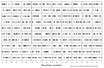
Figure 24: Dot plots of 100 random samples of size \(n=10\) from the \(\mathrm{U}(0,1)\) distribution.
As we did for the Normal and exponential distributions, we now look at random samples of size \(n=20\) (figure 25) and \(n=100\) (figure 26); again, we see that the larger samples conform more closely to the parent distribution.
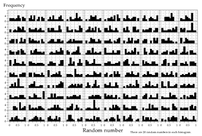
Figure 25: Histograms of 100 random samples of size \(n=20\) from the \(\mathrm{U}(0,1)\) distribution.
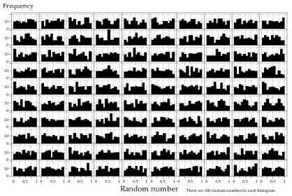
Figure 26: Histograms of 100 random samples of size \(n=100\) from the \(\mathrm{U}(0,1)\) distribution.
Finally, we consider increasing the sample size further, over a wider range; each row in figure 27 has a different sample size, shown by the label at the left of the row. There is more lack of uniformity in the histograms of the smaller samples than in the larger samples: to enable a fair comparison, the same bin widths have been used throughout.
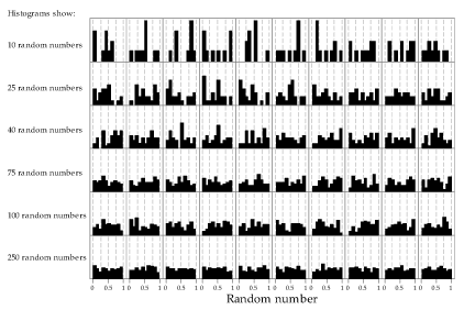
Figure 27: Histograms of random samples of varying size from the \(\mathrm{U}(0,1)\) distribution. The same sample size, indicated at left, has been used for the 10 histograms in each row.
Next page - Content - Sampling from the binomial distribution
| This publication is funded by the Australian Government Department of Education, Employment and Workplace Relations |
Contributors Term of use |