Content
Sampling from exponential distributions
In this section, we look at random samples from exponential distributions. The sequence of diagrams is similar to that in the previous section Sampling from Normal distributions.
A very important message is that there are general features here that are the same as the Normal case. Of course, the shape of the exponential distribution is quite different from the Normal distribution, and hence the distributions of the random samples, shown in the dotplots and histograms, reflect that. However, other features apply regardless of the underlying distribution. For example, with very large sample sizes, the distributions of the samples tend to look like the parent distribution from which the samples are taken: in this case, the exponential distribution.
For this reason, much of the discussion from the previous section Sampling from Normal distributions applies here, and is therefore not repeated in detail.
So that the discussion has a suitable context, we use an example from the module Exponential and normal distributions .. In the example, it is assumed that the underlying random variable represents the interval between births at a country hospital, for which the average time between births is seven days. We assume the distribution of the time between births follows an exponential distribution.
Recall from the module Exponential and normal distributions that, if the random variable \(T\) has an exponential distribution with rate \(\alpha\), which we write as \(T \stackrel{\mathrm{d}}{=} \exp(\alpha)\), then \(T\) has the following pdf:
\[ f_T(t) = \begin{cases} \alpha e^{-\alpha t} &\text{if \(t > 0\),}\\ 0 &\text{otherwise.} \end{cases} \]Moreover, \(\mathrm{E}(T) = \dfrac{1}{\alpha}\). So, if we are using a time unit of days and the mean is seven days, this implies that \(\alpha = \dfrac{1}{7}\).
We take a random sample of size \(n\) from this distribution. In the context of the example, this could be considered a consecutive sequence of \(n\) births, assuming that the times between successive births are independent. (Obviously, multiple births violate this assumption, but we may deal with this by defining a 'birth' to be a birth event to one mother at one time, so that twins and other multiple births count as one 'birth' for these purposes.) It is important to keep in mind that, as usual, the model used is only intended to give some context, and it is an idealised representation with assumptions.
Figures 13 to 15 show three independent random samples from the \(\exp(\dfrac{1}{7})\) distribution. Note the variation between them.
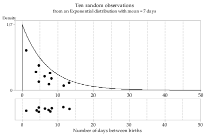
Figure 13: First random sample of size \(n=10\) from the \(\exp(\dfrac{1}{7})\) distribution.

Figure 14: Second random sample of size \(n=10\) from the \(\exp(\dfrac{1}{7})\) distribution.
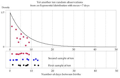
Figure 15: Third random sample of size \(n=10\) from the \(\exp(\dfrac{1}{7})\) distribution.
Figure 16 shows the distributions of 100 random samples, each of size \(n=10\), from the \(\exp(\dfrac{1}{7})\) distribution. The dotplots have been 'jittered' slightly and randomly in the vertical direction to assist with the detection of points that are very close to each other.
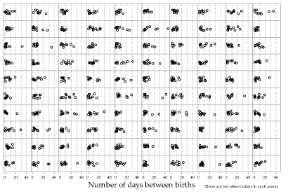
Figure 16: Dotplots of 100 random samples of size \(n=10\) from the \(\exp(\dfrac{1}{7})\) distribution.
Among the first three random samples of size 10, there was no single observation greater than 15 days. Among the 100 random samples of size 10, there are quite a few intervals of greater than 15 days, and one greater than 40 days. This gives another perspective on the simple point that samples vary. If some of the values in the parent population are unlikely, they will — correspondingly — not occur very often in random samples. But if we take enough samples, an unusual individual value will be likely to 'turn up' eventually.
What happens if the sample size is larger? Figures 17 and 18 show 100 histograms (in each case) for random samples of size \(n=20\) (figure 17) and \(n=100\) (figure 18) from the \(\exp(\dfrac{1}{7})\) distribution. Note that the histograms in figure 18 tend to be closer to the shape of the parent distribution.
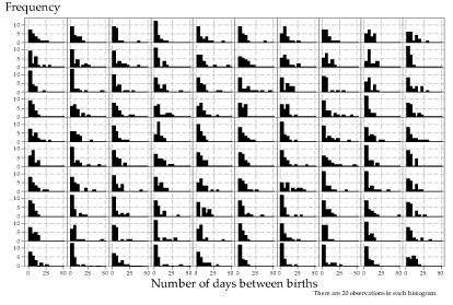
Figure 17: Histograms of 100 random samples of size \(n=20\) from the \(\exp(\dfrac{1}{7})\) distribution.
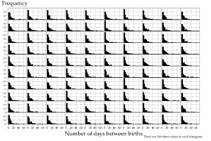
Figure 18: Histograms of 100 random samples of size \(n=100\) from the \(\exp(\dfrac{1}{7})\) distribution.
Figure 19 explores more extensively the effect of varying sample sizes. As we saw for sampling from the Normal distribution, as the sample size increases the histogram becomes more and more similar to the underlying exponential distribution. Looking across the rows, the histograms are more similar to the other histograms (in the same row) for larger sample sizes.
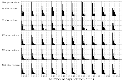
Figure 19: Histograms of random samples of varying size from the \(\exp(\dfrac{1}{7})\) distribution. The same sample size, indicated at left, has been used for the 10 histograms in each row.
Finally, figure 20 shows samples from a number of exponential distributions with different means. Recall that the mean \(\mu\) for an exponential random variable is equal to \(\dfrac{1}{\alpha}\).
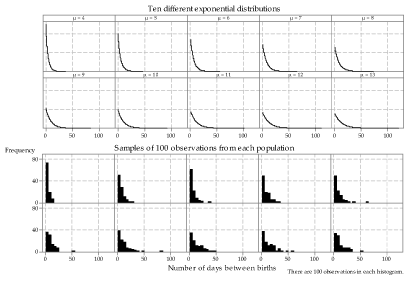
Figure 20: Random samples from different exponential distributions.
Next page - Sampling from the continuous uniform distribution
| This publication is funded by the Australian Government Department of Education, Employment and Workplace Relations |
Contributors Term of use |