Content

Sampling from Normal distributions

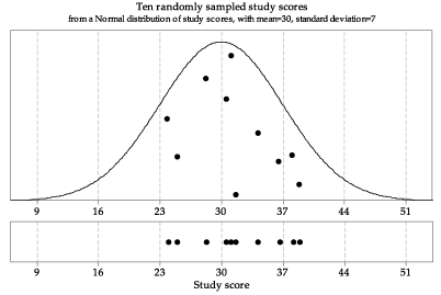
Normal distributions are introduced in the module Exponential and normal distributions . Suppose we are sampling from a Normal population with mean \(\mu=30\) and standard deviation \(\sigma=7\). For example, we could use this distribution to model the population of study scores of Year 12 students in a given subject.

This underlying distribution is shown in figure 4. Also shown is a random sample of size \(n=10\) from this distribution. The 10 observations making up the random sample are superimposed on the probability density function (pdf), to indicate that they come from this distribution. Any single one of the observations is more likely to be a value where the pdf is greater, than where it is smaller. Recall from the module Continuous probability distributions that, for such a random variable \(X\), \(\Pr(X \approx x) \approx f_X(x)\,\delta x\), where \(f_X\) is the pdf of \(X\) and we interpret \(X \approx x\) as the event that \(X\) is in a small interval of width \(\delta x\) around \(x\). For example, if \(f_X(x_1) = 3f_X(x_2)\), then an observation near \(x_1\) is approximately three times more probable than an observation near \(x_2\). This phenomenon is reflected visually in figure 4, in which the observations shown in the pdf are the dots 'floating' above the \(x\)-axis: there is more room for dots above \(x\)-values where the pdf is greater.

Equivalently, we can think of the sample as being obtained by considering the \(x\)--\(y\) plane and choosing \(n\) points randomly from the region under the curve: \(\{\, (x,y): 0 < y < f_X(x) \,\}\), where \(f_X(x)\) is the pdf of \(X\).

A connection with figures 1, 2 and 3 is useful. We can think of figure 4 as containing an infinite pile of marbles in the shape of the region under the curve: the black ones are the ones that happen to be selected.

Detailed description

Figure 4: First random sample of size \(n=10\) from \(\mathrm{N}(30, 7^2)\).

The sample has been projected down to the \(x\)-axis in the lower part of figure 4 to give a dotplot of the data. Recall that a dotplot is a simple way to show the distribution of a small sample.

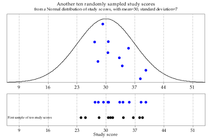
Figure 5 shows another random sample of size 10 from the same parent Normal distribution \(\mathrm{N}(30, 7^2)\). This illustrates the utterly basic but fundamentally important point that repeated samples from the same distribution are different from each other. This is obvious, since they are made up of individual observations from the population distribution, and we know that individual observations vary. Nonetheless, it is an important lesson to absorb; students who are accustomed to the deterministic reproducibility of mathematical relations may find this uncertainty disconcerting.

To make the point about this sample-to-sample variation, both the first and second samples are shown in the lower part of figure 5.

Detailed description

Figure 5: A second random sample of size \(n=10\) from \(\mathrm{N}(30, 7^2)\).

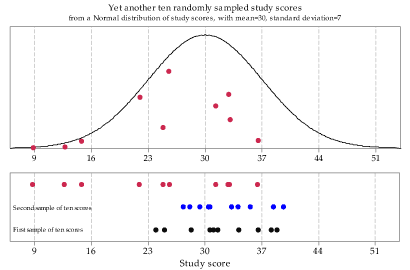
For good measure, figure 6 shows a third sample from the same underlying Normal distribution \(\mathrm{N}(30, 7^2)\), with lined up dotplots of the three random samples.

Detailed description

Figure 6: A third random sample of size \(n=10\) from \(\mathrm{N}(30, 7^2)\).

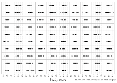
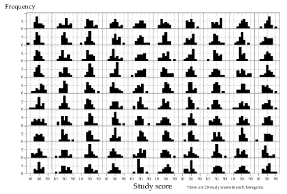
Now we will abandon the visual representation of the underlying Normal distribution \(\mathrm{N}(30, 7^2)\), in order to present a large number of samples of size 10 from this distribution. Figure 7 shows 100 samples of size 10 from this distribution. The choice of 100 as the number to show is arbitrary; all that is intended is to show a large enough number to get an idea of how much variation there can be among such samples. Note the extent of the differences between the samples in both location and spread.

Detailed description

Figure 7: Dotplots of 100 random samples of size \(n=10\) from \(\mathrm{N}(30, 7^2)\).

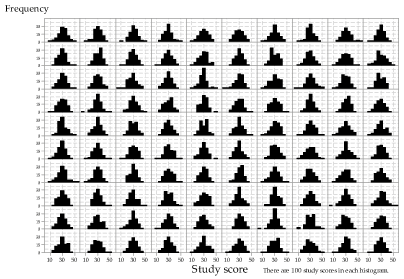
Now we begin to consider the effect of a larger sample size. Figure 8 shows histograms (not dotplots) from 100 random samples of size 20 from the same underlying distribution \(\mathrm{N}(30, 7^2)\). The same \(x\)- and \(y\)-scales are used throughout. Notice how much variation there can be: some look reasonably symmetric and unimodal, while others have marked skewness; some look relatively flat. But all are random samples on \(\mathrm{N}(30, 7^2)\). Remember that a random sample is defined by how it was chosen, and not what it consists of.

Detailed description

Figure 8: Histograms of 100 random samples of size \(n=20\) from \(\mathrm{N}(30, 7^2)\).

What happens if we increase the sample size to 100? This is illustrated in figure 9.

A careful comparison of figures 8 and 9 shows that the histograms in figure 9 are less variable, and closer to the shape of the underlying distribution, than in figure 8. However, even for \(n=100\), there is quite a lot of variation between the random samples from the same distribution.

Detailed description

Figure 9: Histograms of 100 random samples of size \(n=100\) from \(\mathrm{N}(30, 7^2)\).

To get a clearer picture of what happens as the sample size \(n\) increases, figure 10 shows histograms from samples of very different sizes, from \(n=25\) in the first row through to \(n=10\ 000\) in the last row. To facilitate comparisons, the same 'bin widths' and \(y\)-axis scale have been used throughout. Unlike the previous figures, there are 10 histograms for each sample size.

This figure shows clearly that, as the sample size increases, the histogram becomes more and more similar to the underlying distribution. Looking across the rows, the histograms are more similar to the other histograms (in the same row) for larger sample sizes.

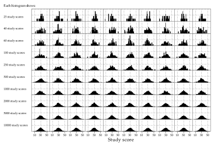
Detailed description

Figure 10: Histograms of random samples of varying size from \(\mathrm{N}(30, 7^2)\). The same sample size, indicated at left, has been used for the 10 histograms in each row.

The same Normal distribution has been used in all cases so far, namely \(\mathrm{N}(30, 7^2)\). Figure 11 illustrates sampling from Normal distributions with different means and standard deviations. In the upper part of the figure, the pdfs of 25 Normal distributions are shown. Each column has the same mean \(\mu\), shown by the label at the top of the column; each row has the same standard deviation \(\sigma\), shown by the label at the left of the row.

In the lower part of the figure, histograms of random samples from the corresponding distributions are shown; the row and column position of the histogram corresponds to that of the distribution from which it came. The same sample size \(n = 100\) has been used throughout. Note how the location and spread of the samples reflect the location and spread of the parent distributions. The locations of the histograms increases from left to right, 'tracking' what happens with the mean \(\mu\). Similarly, the spread of the histograms increases from top to bottom, following the standard deviation \(\sigma\).

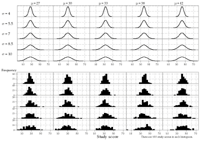
Detailed description

Figure 11: 25 different Normal distributions (upper part) and corresponding histograms of random samples from each of them (lower part); the same sample size \(n=100\) has been used throughout, and the same scales and bin widths have been used in all histograms.

There is a clear link between a pdf in the upper part of figure 11 and the corresponding histogram in the lower part. This suggests that we may be able to make reasonable inferences about the location and spread of a Normal distribution based on a random sample from that distribution when we are not 'given' the pdf. This reasoning is at the heart of statistical inference. The next exercise explores this further.

Detailed description

Figure 12: 25 different Normal distributions (upper part; five are missing) and histograms of random samples from each of them (lower part); the same sample size \(n=100\) has been used throughout.

Next page - Content - Sampling from exponential distributions