Content

Sampling from an infinite population

So far we have been considering the first of the two cases of random sampling: sampling from a finite population. We now consider the second case: sampling from an infinite population.

The whole idea of an infinite population is clearly quite abstract. One way to think of it is to consider sampling from a finite population, and increasing the size of the population: suppose that the population size \(N\) tends to infinity. Sampling from an infinite population is handled by regarding the population as represented by a distribution. A random sample from an infinite population is therefore considered as a random sample from a distribution.

This means that there is an underlying distribution governing the random sample, typically making some values more likely than others, according to the shape of the distribution. The underlying distribution can be thought of as the distribution of some random variable \(X\).

A random sample 'on \(X\)' of size \(n\) is defined to be \(n\) random variables \(X_1,X_2,\dots,X_n\) that are mutually independent and have the same distribution as \(X\).

Over the remainder of this module, we discuss samples from different distributions. The approach is strongly visual, using diagrams to convey the important ideas.

The relevant distribution is not arbitrary: it is determined from first principles, or by appeal to the pattern in applicable historical data. We may think of the distribution of \(X\) as the underlying or 'parent' distribution, producing \(n\) 'offspring' that make up the random sample.

There are some important features of a random sample defined in this way:

• Any single element of the random sample, \(X_i\), comes from the parent distribution, defined by the distribution of \(X\). The distribution of \(X_i\) is the same as the distribution of \(X\). So the chance that \(X_i\) takes any particular value is determined by the shape and pattern of the distribution of \(X\).
• There is variation between different random samples of size \(n\) from the same underlying population distribution. Appreciating the existence of this variation and understanding it is central to the process of statistical inference, which is considered in the modules Inference for proportions and Inference for means.
• If we take a very large random sample from \(X\), and draw a histogram of the sample, the shape of the histogram will tend to resemble the shape of the distribution of \(X\).
• If \(n\) is small, the evidence from the sample about the shape of the parent distribution will be very imprecise: the sample may be consistent with a number of different parent distributions.
• Independence between the \(X_i\)'s is a crucial feature: if the \(X_i\)'s are not independent, then the features we discuss here may not apply, and often will not apply. And because there are \(n\) random variables, it is mutual independence that is required. This means that the conditional distribution of \(X_j\), given the values of any number of the other \(X_i\)'s (\(i \neq j\)), is the same as the (unconditional) distribution of \(X_j\). No matter what we are told about the other \(X_i\)'s, the distribution of \(X_j\) is unchanged.

A simple random sample from a very large finite population is approximately the same as a random sample from an infinite population. If we draw two numbers at random, without replacement, from a population consisting of the integers \(1,2,3,4,5\), the second number is clearly not independent of the first number. If we define \(A =\) "first number drawn is 3" and \(B =\) "second number drawn is 4", then \(\Pr(B) = \dfrac{1}{5}\), but \(\Pr(B|A) = \dfrac{1}{4}\), and since these two probabilities are not equal, the events are not independent.

On the other hand, if we draw two numbers at random, without replacement, from a population consisting of the integers \(1,2,3,\dots,10\ 000\), then the corresponding events have the following probabilities: \(\Pr(B) = \dfrac{1}{10\ 000}\), but \(\Pr(B|A) = \dfrac{1}{9999}\). These are different, so the two events are not independent, but they are very close, so the events in this case are approximately independent: \(\Pr(B) \approx \Pr(B|A)\).

This point is illustrated as follows. Consider the following population of 100 numbers; the population distribution is shown. Think of them as marbles with numbers marked on them, positioned at the point corresponding to their number.

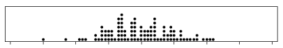
Figure 1: The distribution of a finite population of size \(N=100\).

Imagine selecting one of these marbles at random. This affects the population, perhaps noticeably: the removed marble is apparent. If a random sample of size \(n=50\) is taken from this population, it changes the population markedly: there is only half of the population left.

Now consider a much larger population of marbles with numbers on them: for example, \(N=10\ 000\) (see figure 2). Removing one marble at random would not be noticeable; even taking a random sample of size \(n=50\) from this population will hardly change it all.

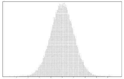
Figure 2: The distribution of a finite population of size \(N=10\ 000\).

Finally, imagine a huge population — think \(N=10^{100}\). Now the population is so vast that the marbles are essentially infinitesimally small (see figure 3).

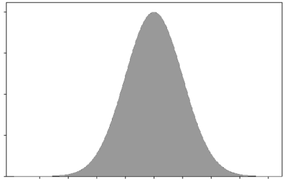
Figure 3: The distribution of a population of huge size.

Each time a marble is selected (from this 'infinite' pile of marbles), it will effectively be a selection from this distribution, no matter what other marbles have been selected. That is, each observation has the distribution shown in figure 3, independently of the other observations.

Next page - Content - Sampling from Normal distributions