Content

Conditional probability

Like many other basic ideas of probability, we have an intuitive sense of the meaning and application of conditional probability from everyday usage, and students have seen this in previous years.

Suppose the chance that I leave my keys at home and arrive at work without them is 0.01. Now suppose I was up until 2 a.m. the night before, had to hurry in the morning, and used a different backpack from my usual one. What then is the chance that I don't have my keys? What we are given — new information about what has occurred — can change the probability of the event of interest. Intuitively, the more difficult circumstances of the morning described will increase the probability of forgetting my keys.

Consider the probability of obtaining 2 when rolling a fair die. We know that the probability of this outcome is \(\dfrac{1}{6}\). Suppose we are told that an even number has been obtained. Given this information, what is the probability of obtaining 2? There are three possible even-number outcomes: 2, 4 or 6. These are equiprobable. One of these three outcomes is 2. So intuition tells us that the probability of obtaining 2, given that an even number has been obtained, is \(\dfrac{1}{3}\). Similar reasoning leads to the following: The probability of obtaining 2, given that an odd number has been obtained, equals zero. If we know that an odd number has been obtained, then obtaining 2 is impossible, and hence has conditional probability equal to zero.

Using these examples as background, we now consider conditional probability formally. When we have an event \(A\) in a random process with event space \(\mathcal{E}\), we have used the notation \(\Pr(A)\) for the probability of \(A\). As the examples above show, we may need to change the probability of \(A\) if we are given new information that some other event \(D\) has occurred. Sometimes the conditional probability may be larger, sometimes it may be smaller, or the probability may be unchanged: it depends on the relationship between the events \(A\) and \(D\).

We use the notation \(\Pr(A|D)\) to denote `the probability of \(A\) given \(D\)'. We seek a way of finding this conditional probability.

It is worth making the observation that, in a sense, all probabilities are conditional: the condition being (at least) that the random process has occurred. That is, it is reasonable to think of \(\Pr(A)\) as \(\Pr(A|\mathcal{E})\).

It helps to think about conditional probability using a suitable diagram, as follows.

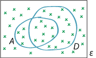
Illustrating conditional probability.

If the event \(D\) has occurred, then the only elementary events in \(A\) that can possibly have occurred are those in \(A \cap D\). The greater (or smaller) the probability of \(A \cap D\), the greater (or smaller) the value of \(\Pr(A|D)\). Logic dictates that \(\Pr(A|D)\) should be proportional to \(\Pr(A \cap D)\). That is,

\[ \Pr(A|D) = c \times \Pr(A \cap D), \] for some constant \(c\) determined by \(D\).

We are now in a new situation, where we only need to consider the intersection of events with \(D\); it is as if we have a new, reduced event space. We still want to consider the probabilities of events, but they are all revised to be conditional on \(D\), that is, given that \(D\) has occurred.

The usual properties of probability should hold for \(\Pr( \,\cdot\, |D)\). In particular, the second axiom of probability tells us that we must have \(\Pr(\mathcal{E}|D) = 1\). Hence

\[ 1 = \Pr(\mathcal{E}|D) = c \Pr(\mathcal{E} \cap D) = c \Pr(D), \] which implies that \[ c = \dfrac{1}{\Pr(D)}. \]

We have obtained the rule for conditional probability: the probability of the event \(A\) given the event \(D\) is

\[ \Pr(A|D) = \dfrac{\Pr(A \cap D)}{\Pr(D)}. \]

Since \(\Pr(D)\) is the denominator in this formula, we are in trouble if \(\Pr(D) = 0\); we need to exclude this. However, in the situations we consider, if \(\Pr(D) = 0\), then \(D\) cannot occur; so in that circumstance it is going to be meaningless to speak of any probability, given that \(D\) has occurred.

We can rearrange this equation to get another useful relationship, sometimes known as the multiplication theorem:

\[ \Pr(A \cap D) = \Pr(D) \times \Pr(A|D). \]

We can interchange \(A\) and \(D\) and also obtain

\[ \Pr(A \cap D) = \Pr(A) \times \Pr(D|A). \]

This is now concerned with the probability conditional on \(A\).

Next page - Content - Independence