Content
The law of total probability
We saw in the traffic-lights example from the previous section that it can be convenient to calculate the probability of an event in a somewhat indirect manner, by summing probabilities involving intersections. We now consider that process in more detail.
Events \(A_1, A_2, \dots, A_k\) are said to be a partition of the event space if they are mutually exclusive and their union is the event space \(\mathcal{E}\). That is, if events \(A_1, A_2, \dots, A_k\) are such that
- \(A_i \cap A_j = \varnothing\), for all \(i \ne j\), and
- \(A_1 \cup A_2 \cup \dots \cup A_k = \mathcal{E}\),
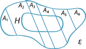
A partition of the event space and the intersection of an event \(H\) with the partition.
Detailed description
The simplest version of a partition is any event \(A\) and its complement, since \(A \cap A' = \varnothing\) and \(A \cup A' = \mathcal{E}\).
Note the event \(H\) represented on the diagram of the event space \(\mathcal{E}\) above. It appears from the diagram that the probability of \(H\) can be obtained by summing the probabilities of the intersection of \(H\) with each event \(A_i\) in the partition. We can show this formally:
\begin{align*} H &= H \cap \mathcal{E}\\ &= H \cap (A_1 \cup A_2 \cup \dots \cup A_k)\\ &= (H \cap A_1) \cup (H \cap A_2) \cup \dots \cup (H \cap A_k). \end{align*}Since \(A_1, A_2, \dots, A_k\) are mutually exclusive, it follows that the events
\[ H \cap A_1, \ H \cap A_2, \ \dotsc, \ H \cap A_k \] are also mutually exclusive. Hence, by the third axiom of probability, \begin{align*} \Pr(H) &= \Pr(H \cap A_1) + \Pr(H \cap A_2) + \dots + \Pr(H \cap A_k)\\ &= \Pr(A_1)\Pr(H|A_1) + \Pr(A_2)\Pr(H|A_2) + \dots + \Pr(A_k)\Pr(H|A_k)\\ &= \sum_{i=1}^{k} \Pr(A_i)\Pr(H|A_i). \end{align*}This result is known as the law of total probability. Note that it does not matter if there are some events \(A_j\) in the partition for which \(H \cap A_j = \varnothing\). (For example, see \(A_1\) and \(A_6\) in the diagram above.) For these events, \(\Pr(H \cap A_j) = 0\).
A table can provide a useful alternative way to represent the partition and the event \(H\) shown in the diagram above. In the following table, the event \(A_3\) is used as an example.
| \(H\) | \(H'\) | ||
| \(A_1\) | \(\Pr(A_1)\) | ||
| \(A_2\) | \(\Pr(A_2)\) | ||
| \(A_3\) | \(\Pr(A_3 \cap H) = \Pr(A_3)\Pr(H|A_3) \) | \(\Pr(A_3)\) | |
| \(A_4\) | \(\Pr(A_4)\) | ||
| \(A_5\) | \(\Pr(A_5)\) | ||
| \(A_6\) | \(\Pr(A_6)\) | ||
| \(\Pr(H)\) | \(\Pr(H')\) |
Example: Traffic lights, continued
We have seen an illustration of the law of total probability, in the traffic-lights example from the previous section. We obtained the probability of the rider meeting green at the second set of traffic lights by using the possible events at the first set of traffic lights, \(G_1\) and \(R_1\). These two events are a partition: note that \(R_1 = G'_1\). Hence,
\begin{align*} \Pr(G_2) &= \Pr(G_1 \cap G_2) + \Pr(R_1 \cap G_2)\\ &= \Pr(G_1) \Pr(G_2|G_1) + \Pr(R_1) \Pr(G_2|R_1)\\ &= (0.3 \times 0.6) + (0.7 \times 0.4)\\ &= 0.18 + 0.28\\ &= 0.46. \end{align*}In contexts with sequences of events, for which we use tree diagrams, we may be interested in the conditional probability of an event at the first stage, given what happened at the second stage. This is a reversal of what seems to be the natural order, but it is sometimes quite important. In the traffic-lights example, it would mean considering a conditional probability such as \(\Pr(G_1|G_2)\): the probability that the rider encounters green at the first set of traffic lights, given that she encounters green at the second set.
Again, consider the general situation involving a partition \(A_1, A_2, \dots, A_k\) and an event \(H\). The law of total probability enables us to find \(\Pr(H)\) from the probabilities \(\Pr(A_i)\) and \(\Pr(H|A_i)\). However, we may be interested in \(\Pr(A_i|H)\). This is found using the standard rule for conditional probability:
\[ \Pr(A_i|H) = \dfrac{\Pr(A_i \cap H)}{\Pr(H)}. \]We can use the multiplication theorem in the numerator and the law of total probability in the denominator to obtain
\[ \Pr(A_i|H) = \dfrac{\Pr(A_i) \Pr(H|A_i)}{\sum_{j=1}^{k} \Pr(A_j)\Pr(H|A_j)}. \]This process involves a `reversal' of the conditional probabilities.
It is most important to avoid confusion between the two possible conditional probabilities: Are we thinking of \(\Pr(C|D)\) or \(\Pr(D|C)\)? The language of any conditional probability statement must be examined closely to get this right.
These ideas are applied in diagnostic testing for diseases, as illustrated by the following example.
Example: Diagnostic testing
Suppose that a diagnostic screening test for breast cancer is used in a population of women in which 1% of women actually have breast cancer. Let \(C\) = "woman has breast cancer", so that \(\Pr(C) = 0.01\). Suppose that the test finds that a woman has breast cancer, given that she actually does, in 85% of such cases. Let \(T_{+}\) = "test is positive, that is, indicates cancer"; then \(\Pr(T_{+}|C) = 0.85\). This quantity is known in diagnostic testing as the sensitivity of the test.
Suppose that when a woman actually does not have cancer, the test gives a negative result (indicating no cancer) in 93% of such cases; that is, \(\Pr(T_{-}|C') = 0.93\). This is called the specificity of the test.
Clearly, we want both the sensitivity and the specificity to be as close as possible to 1.0. But — particularly for relatively cheap screening tests — this cannot always be achieved. (You may wonder how the sensitivity and specificity of such a diagnostic test can ever be determined, or estimated. This is done by using definitive tests of the presence of cancer, which may be much more invasive and costly than the non-definitive test under scrutiny. The non-definitive test can be applied in a large group of women whose cancer status is clear, one way or the other, to estimate the sensitivity and specificity.)
Before reading further, try to guess how likely it is that a woman (from this population) who tests positive on this test actually has cancer?
People's intuition on this question is often alarmingly awry. Notice that this is a question of genuine interest and concern in practice: the screening program will need to follow up with women who test positive, leading to more testing and also to obvious concern on the part of these women.
This crucial clinical question is: What is \(\Pr(C|T_{+})\)?
This is a natural context for a tree diagram, which is shown below. This is because there are two stages. The first stage concerns whether or not the woman has cancer, and the second stage is the result of the test, positive (indicating cancer) or not. We find, for example, that \(\Pr(T_{+} \cap C) = \Pr(C) \Pr(T_{+}|C) = 0.01 \times 0.85 = 0.0085\).
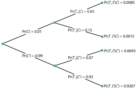
Tree diagram for the diagnostic-testing example.
Detailed description
We can now apply the usual rule for conditional probability to find \(\Pr(C|T_{+})\):
\[ \Pr(C|T_{+}) = \dfrac{\Pr(C \cap T_{+})}{\Pr(T_{+})} = \dfrac{0.0085}{\Pr(T_{+})}. \]To find \(\Pr(T_{+})\), we use the law of total probability:
\begin{align*} \Pr(T_{+}) &= \Pr(C \cap T_{+}) + \Pr(C' \cap T_{+})\\ &= \Pr(C) \Pr(T_{+}|C) + \Pr(C') \Pr(T_{+}|C')\\ &= (0.01 \times 0.85) + (0.99 \times 0.07)\\ &= 0.0085 + 0.0693\\ &= 0.0778. \end{align*}Hence
\[ \Pr(C|T_{+}) = \dfrac{\Pr(C \cap T_{+})}{\Pr(T_{+})} = \dfrac{0.0085}{0.0778} \approx 0.1093. \]Note what this implies: Among women with positive tests (indicating cancer), about 11% actually do have cancer. This is known as the positive predictive value. Many people are surprised by how low this probability is. Women who actually do have cancer and test positive are known as true positives. In this example, the overwhelming majority (about 89%) of women with a positive test do not have cancer; women who do not have cancer but who test positive are known as false positives.
The information in the tree diagram can also be represented in a table, as follows.
| \(T_+\) | \(T_-\) | ||
| \(C\) | \(\Pr(C \cap T_+) = 0.0085\) | \(\Pr(C \cap T_-) = 0.0015\) | \(\Pr(C)=0.01\) |
| \(C'\) | \(\Pr(C' \cap T_+) = 0.0693\) | \(\Pr(C' \cap T_-) = 0.9207\) | \(\Pr(C')=0.99\) |
| \(\Pr(T_+) = 0.0778\) | \(\Pr(T_-) = 0.9222\) |
Exercise 13
Consider the diagnostic-testing example above.
- Find \(\Pr(C'|T_{-})\). This quantity is known as the negative predictive value: it concerns true negatives, that is, women who do not have cancer and who have a negative test.
- For \(\Pr(C) = 0.01\) and \(\Pr(T_{-}|C')=0.93\), as in the example, what is the largest possible value for the positive predictive value \(\Pr(C|T_{+})\)?
- For \(\Pr(C) = 0.01\) and \(\Pr(T_{+}|C)=0.85\), as in the example, what value of the specificity \(\Pr(T_{-}|C')\) gives a positive predictive value \(\Pr(C|T_{+})\) of:
- 0.20
- 0.50
- 0.80
- 0.99?
- Breast cancer is many times rarer in men than in women. Suppose that a population of men are tested with the same test, and that the same sensitivity and specificity apply (so \(\Pr(T_{+}|C)=0.85\) and \(\Pr(T_{-}|C')=0.93\)), but that in men \(\Pr(C) = 0.0001\). Find \(\Pr(C|T_{+})\) and \(\Pr(C'|T_{-})\).
Next page - Answers to exercises
| This publication is funded by the Australian Government Department of Education, Employment and Workplace Relations |
Contributors Term of use |