Content
Newton's method
Truth is much too complicated to allow anything but approximations.
— John Von Neumann
Finding a solution with geometry
Newton's method for solving equations is another numerical method for solving an equation $f(x) = 0$. It is based on the geometry of a curve, using the tangent lines to a curve. As such, it requires calculus, in particular differentiation.
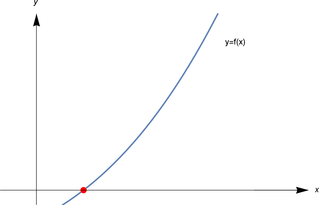
Roughly, the idea of Newton's method is as follows. We seek a solution to $f(x) = 0$. That is, we want to find the red dotted point in the picture below.
We start with an initial guess $x_1$. We calculate $f(x_1)$. If $f(x_1) = 0$, we are very lucky, and have a solution. But most likely $f(x_1)$ is not zero. Let $f(x_1) = y_1$, as shown.
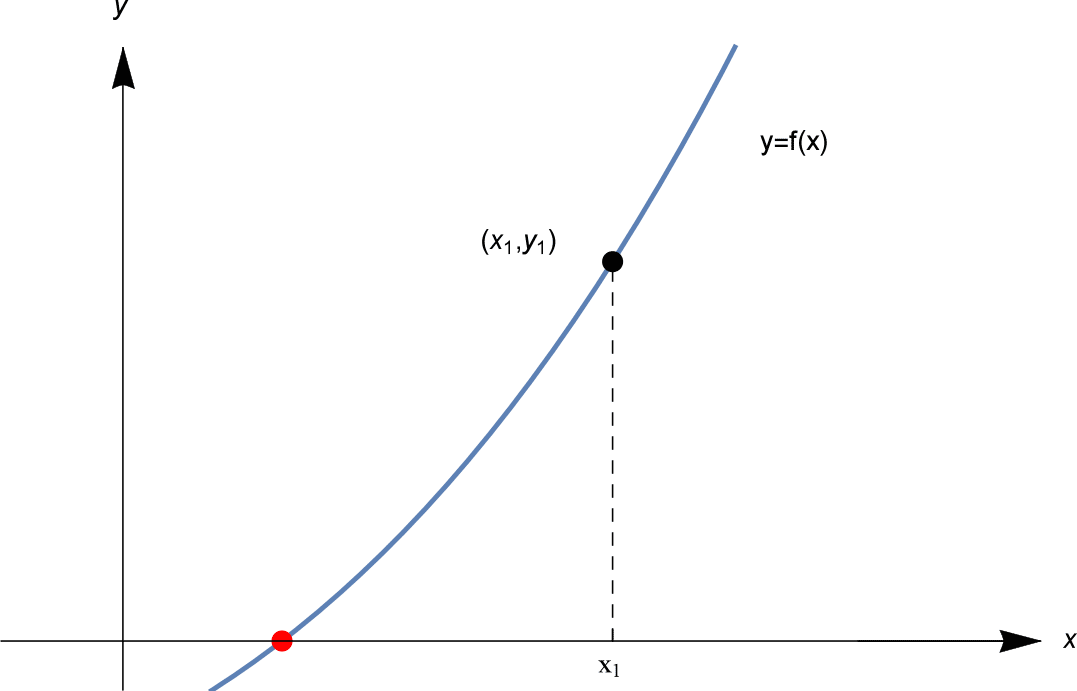
We now try for a better guess. How to find that better guess? The trick of Newton's method is to draw a tangent line to the graph $y=f(x)$ at the point $(x_1, y_1)$. See below.
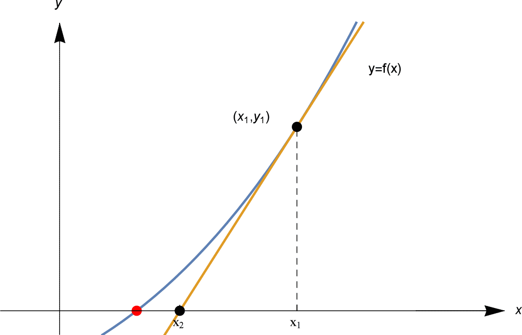
This tangent line is a good linear approximation to $f(x)$ near $x_1$, so our next guess $x_2$ is the point where the tangent line intersects the $x$-axis, as shown above.
We then proceed using the same method. We calculate $y_2 = f(x_2)$; if it is zero, we're finished. If not, then we draw the tangent line to $y=f(x)$ at $(x_2, y_2)$, and our next guess $x_3$ is the point where this tangent line intersects the $x$-axis. See below.
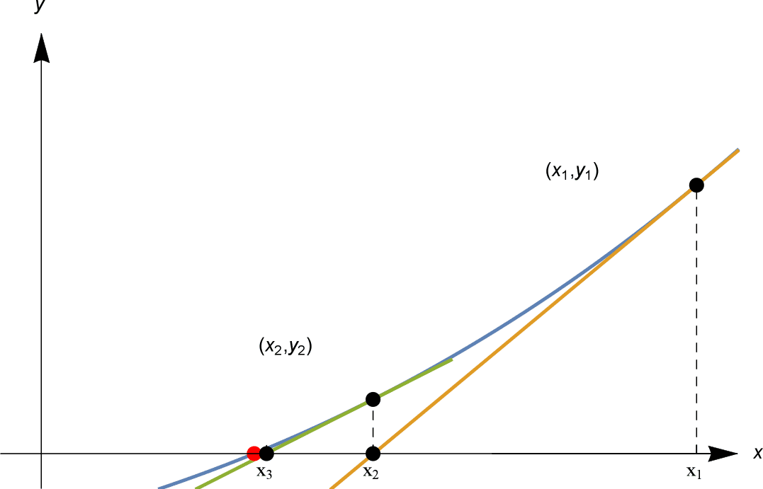
In the figure shown, $x_1, x_2, x_3$ rapidly approach the red solution point!
Continuing in this way, we find points $x_1, x_2, x_3, x_4, \ldots$ approximating a solution. This method for finding a solution is Newton's method.
As we'll see, Newton's method can be a very efficient method to approximate a solution to an equation — when it works.
The key calculation
As our introduction above just showed, the key calculation in each step of Newton's method is to find where the tangent line to $y=f(x)$ at the point $(x_1, y_1)$ intersects the $x$-axis.
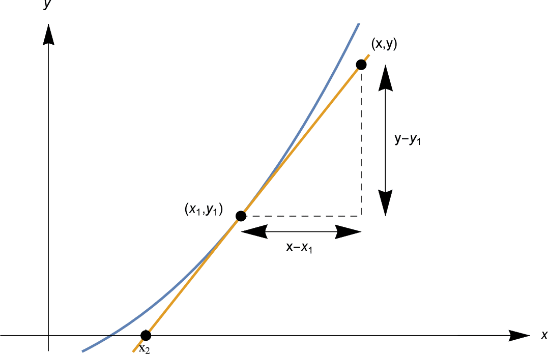
Let's find this $x$-intercept. The tangent line we are looking for passes through the point $(x_1, y_1)$ and has gradient $f'(x_1)$.
Recall that, given the gradient $m$ of a line, and a point $(x_0, y_0)$ on it, the line has equation
\[ \frac{y-y_0}{x-x_0} = m, \quad \text{or equivalently,} \quad y = m(x-x_0) + y_0. \]In our situation, the line has gradient $f'(x_1)$, and passes through $(x_1, y_1)$, so has equation
\[ \frac{y-y_1}{x-x_1} = f'(x_1), \quad \text{or equivalently,} \quad y = f'(x_1) (x-x_1) + y_1. \]See the diagram below.
Setting $y=0$, we find the $x$-intercept as
\[ x = x_1 - \frac{y_1}{f'(x_1)} = x_1 - \frac{f(x_1)}{f'(x_1)}. \]The Algorithm
We can now describe Newton's method algebraically. Starting from $x_1$, the above calculation shows that if we construct the tangent line to the graph $y=f(x)$ at $x=x_1$, this tangent line has $x$-intercept given by
\[ x_2 = x_1 - \frac{f(x_1)}{f'(x_1)}. \]Then, starting from $x_2$ we perform the same calculation, and obtain the next approximation $x_3$ as
\[ x_3 = x_2 - \frac{f(x_2)}{f'(x_2)}. \]The same calculation applies at each stage: so from the $n$'th approximation $x_n$, the next approximation is given by
\[ x_{n+1} = x_n - \frac{f(x_n)}{f'(x_n)}. \]Formally, Newton's algorithm is as follows.
Newton's method
Let $f: \mathbb{R} \rightarrow \mathbb{R}$ be a differentiable function. We seek a solution of $f(x) = 0$, starting from an initial estimate $x = x_1$.
At the $n$'th step, given $x_n$, compute the next approximation $x_{n+1}$ by
\[ x_{n+1} = x_n - \frac{f(x_n)}{f'(x_n)} \quad \text{and repeat}. \]Some comments about this algorithm:
- Often, Newton's method works extremely well, and the $x_n$ converge rapidly to a solution. However, it's important to note that Newton's method does not always work. Several things can go wrong, as we will see shortly.
- Note that if $f(x_n) = 0$, so that $x_n$ is an exact solution of $f(x) = 0$, then the algorithm gives $x_{n+1} = x_n$, and in fact all of $x_n, x_{n+1}, x_{n+2}, x_{n+3}, \ldots$ will be equal. If you have an exact solution, Newton's method will stay on that solution!
- While the bisection method only requires $f$ to be continuous, Newton's method requires the function $f$ to be differentiable. This is necessary for $f$ to have a tangent line.
Using Newton's method
As we did with the bisection method, let's approximate some well-known constants.
Example
Use Newton's method to find an approximate solution to $x^2 - 2 = 0$, starting from an initial estimate $x_1 =2$. After 4 iterations, how close is the approximation to $\sqrt{2}$?
Solution
Let $f(x) = x^2 - 2$, so $f'(x) = 2x$. At step 1, we have $x_1 = 2$ and we calculate $f(x_1) = 2^2 - 2 = 2$ and $f'(x_1) = 4$, so
\[ x_2 = x_1 - \frac{f(x_1)}{f'(x_1)} = 2 - \frac{2}{4} = \frac{3}{2} = 1.5. \]At step 2, from $x_2 = \frac{3}{2}$ we calculate $f(x_2) = \frac{1}{4}$ and $f'(x_2) = 3$, so
\[ x_3 = x_2 - \frac{f(x_2)}{f'(x_2)} = \frac{3}{2} - \frac{ \frac{1}{4} }{ 3 } = \frac{17}{12} \sim 1.41666667 \quad \text{(to 8 decimal places).} \]At step 3, from $x_3 = \frac{17}{12}$ we have $f(x_3) = \frac{1}{144}$ and $f'(x_3) = \frac{17}{6}$, so
\[ x_4 = x_3 - \frac{f(x_3)}{f'(x_3)} = \frac{17}{12} - \frac{ \frac{1}{144} }{ \frac{17}{6} } = \frac{577}{408} \sim 1.41421569 \quad \text{(to 8 decimal places).} \]At step 4, from $x_4 = \frac{577}{408}$ we calculate $f(x_4) = \frac{1}{166,464}$ and $f'(x_4) = \frac{577}{204}$, so
\[ x_5 = x_4 - \frac{f(x_4)}{f'(x_4)} = \frac{665,857}{470,832} \sim 1.414213562375 \quad \text{(to 12 decimal places).} \]In fact, to 12 decimal places $\sqrt{2} \sim 1.414213562373$. So after 4 iterations, the approximate solution $x_5$ agrees with $\sqrt{2}$ to 11 decimal places. The difference between $x_5$ and $\sqrt{2}$ is
\[ \frac{665,857}{470,832} - \sqrt{2} \sim 1.59 \times 10^{-12} \quad \text{to 3 significant figures.} \]Newton's method in the above example is much faster than the bisection algorithm! In only 4 iterations we have 11 decimal places of accuracy! The following table illustrates how many decimal places of accuracy we have in each $x_n$.
| $n$ | $1$ | $2$ | $3$ | $4$ | $5$ | $6$ | $7$ |
| # decimal places accuracy in | $0$ | $0$ | $2$ | $5$ | $11$ | $23$ | $47$ |
The number of decimal places of accuracy approximately doubles with each iteration!
Exercise 10
(Harder.) This problem investigates this doubling of accuracy:- First calculate that $x_{n+1} = \frac{x_n}{2} + \frac{1}{x_n}$ and that, if $y_n = x_n - \sqrt{2}$, then $y_{n+1} = \frac{y_n^2}{2(\sqrt{2} + y_n)}$.
- Show that, if $x_1 > 0$ (resp. $x_1 < 0$), then $x_n > \sqrt{2}$ (resp. $x_n < - \sqrt{2})$ for all $n \geq 2$.
- Show that if $0 < y_n < 10^{-k}$ for some positive integer $k$, then $0 < y_{n+1} < 10^{-2k}$.
- Show that, for $n \geq 2$, if $x_n$ differs from $\sqrt{2}$ by less than $10^{-k}$, then $x_{n+1}$ differs from $\sqrt{2}$ by less than $10^{-2k}$.
Example
Find an approximation to $\pi$ by using Newton's method to solve $\sin x = 0$ for 3 iterations, starting from $x_1=3$. To how many decimal places is the approximate solution accurate?
Solution
Let $f(x) = \sin x$, so $f'(x) = \cos x$. We compute $x_2, x_3, x_4$ directly using the formula
\[ x_{n+1} = x_n - \frac{f(x_n)}{f'(x_n)} = x_n - \frac{\sin x_n}{\cos x_n} = x_n - \tan x_n. \]We compute directly each $x_n$ to 25 decimal places, for 3 iterations:
\[ \begin{array}{ll} x_2 &= x_1 - \tan x_1 = 3 - \tan 3 \sim 3.1425465430742778052956354 \\ x_3 &= x_2 - \tan x_2 \sim 3.1415926533004768154498858 \\ x_4 &= x_3 - \tan x_3 \sim 3.1415926535897932384626434 \\ \end{array} \]To 25 decimal places, $\pi = 3.1415926535897932384626433$; $x_4$ agrees to 24 places.
In the above example, convergence is even more rapid than for our $\sqrt{2}$ example. The number of decimal places accuracy roughly triples with each iteration!
| $n$ | $1$ | $2$ | $3$ | $4$ | $5$ |
| # decimal places accuracy in $x_n$ | $0$ | $2$ | $9$ | $24$ | $87$ |
Exercise 11
Find all solutions to the equation $\cos x = x$ to 9 decimal places using Newton's method. Compare the convergence to what you obtained with the bisection method in exercise 5.
What can go wrong
While Newton's method can give fantastically good approximations to a solution, several things can go wrong. We now examine some of this less fortunate behaviour.
The first problem is that the $x_n$ may not even be defined!
Example
Find an approximate solution to $\sin x = 0$ using Newton's method starting from $x_1 = \frac{\pi}{2}$.
Solution
We set $f(x) = \sin x$, so $f'(x) = \cos x$. Now $x_2 = x_1 - \frac{f(x_1)}{f'(x_1)}$, but $f'(x_1) = \cos \frac{\pi}{2} = 0$, so $x_2$ is not defined, hence nor are any subsequent $x_n$.
This problem occurs whenever when $f'(x_n) = 0$. If $x_n$ is a stationary point of $f$, then Newton's method attempts to divide by zero — and fails.
The next example illustrates that even when the "approximate solutions" $x_n$ exist, they may not "approximate" a solution very well.
Example
Approximate a solution to $-x^3 + 4x^2 - 2x + 2 = 0$ using Newton's method from $x_1 = 0$.
Solution
Let $f(x) = -x^3 + 4x^2 - 2x + 2$, so $f'(x) = -3x^2 + 8x - 2$. Starting from $x_1 = 0$, we have
\[ x_2 = x_1 - \frac{f(x_1)}{f'(x_1)} = - \frac{f(0)}{f'(0)} = - \frac{2}{-2} = 1, \quad \text{then} \quad x_3 = x_2 - \frac{f(x_2)}{f'(x_2)} = 1 - \frac{f(1)}{f'(1)} = 1 - \frac{3}{3} = 0. \]We have now found that $x_3 = x_1 = 0$. The computation for $x_4$ is then exactly the same as for $x_2$, so $x_4 = x_2 = 1$. Thus $x_n = 0$ for all odd $n$, and $x_n = 1$ for all even $n$. The $x_n$ are locked into a cycle, alternating between two values.
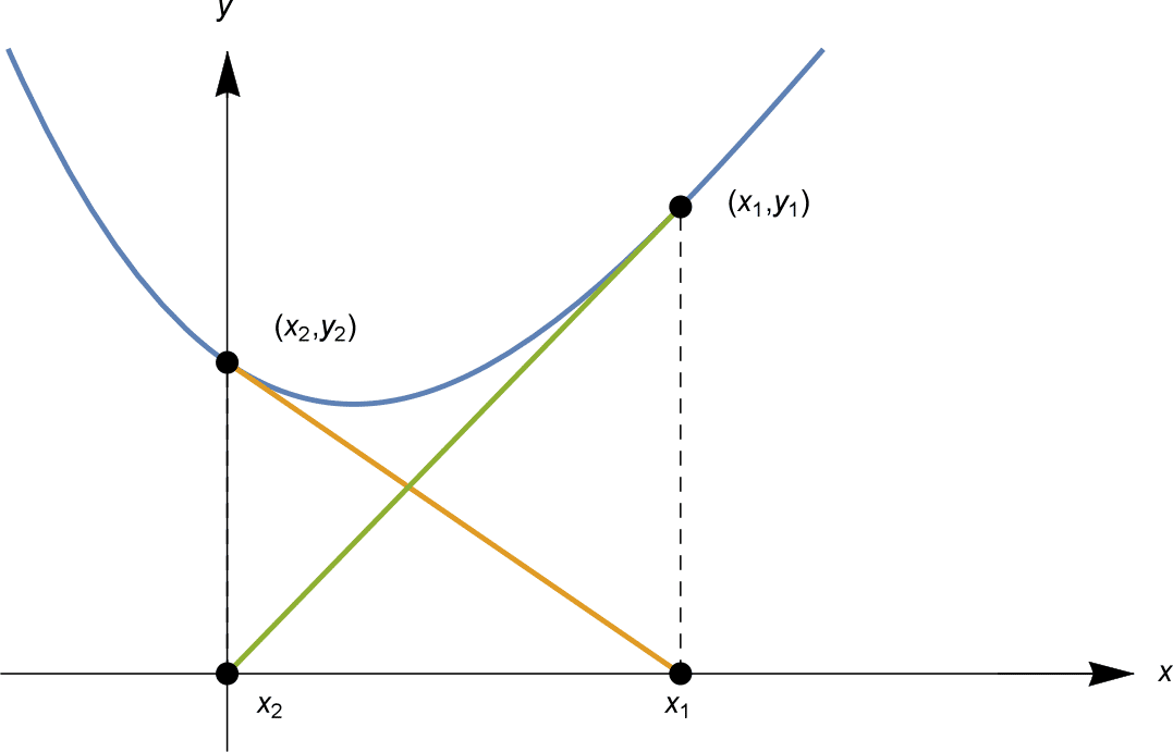
In the above example, there is actually a solution, $x = \frac{1}{3} \left( 4 + \sqrt{10} + \sqrt[3]{100} \right) \sim 3.59867$. Our "approximate solutions" $x_n$ fail to approximate it, instead cycling as illustrated below.
The third problem shows that all $x_n$ can get further and further away from a solution!
Example
Find an approximate solution to $\arctan x = 0$, using Newton's method starting at $x_1 = 3$.
Solution
Let $f(x) = \arctan x$, so $f'(x) = \frac{1}{1+x^2}$. From $x_1 = 3$ we can compute successively $x_2, x_3, \ldots$. We write them to 2 decimal places.
\begin{align*} x_2 &= x_1 - \frac{f(x_1)}{f'(x_1)} = 3 - \frac{\arctan 3}{\frac{1}{1+3^2}} = 3 - 10 \arctan 3 \sim -9.49. \\ x_3 &= x_2 - \frac{f(x_2)}{f'(x_2)} \sim 124.00 \\ x_4 &= x_3 - \frac{f(x_3)}{f'(x_3)} \sim -23,905.94 \end{align*}The "approximations" $x_n$ rapidly diverge to infinity.
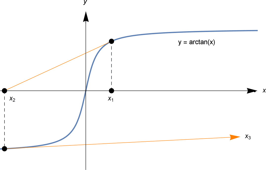
The above example may seem a little silly, since finding an exact solution to $\arctan x = 0$ is not difficult: the solution is $x=0$! But similar problems will happen applying Newton's method to any curve with a similar shape. The fact that $f'(x_n)$ is close to zero means the tangent line is close to horizontal, and so may travel far away to arrive at its $x$-intercept of $x_{n+1}$.
Sensitive dependence on initial conditions
Sometimes the choice of initial conditions can be ever so slight, yet lead to a radically different outcome in Newton's method.
Consider solving $f(x) = 2x - 3x^2 + x^3 = 0$. It's possible to factorise the cubic, $f(x) = x(x-1)(x-2)$, so the solutions are just $x=0, 1$ and $2$.
If we apply Newton's method with different starting estimates $x_1$, we might end up at any of these three solutions... or somewhere else.
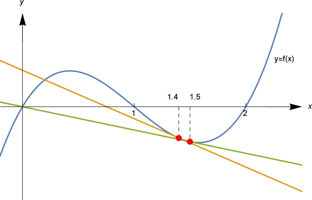
As illustrated above, we apply Newton's method starting from $x_1 = 1.4$ and $x_1 = 1.5$. Starting from $x_1 = 1.4 = \frac{7}{5}$ we compute, to 6 decimal places,
\[ x_1 = \frac{7}{5} = 1.4, \; x_2 \sim 0.753 846, \; x_3 \sim 1.036 456, \; x_4 \sim 0.999 903, \; x_5 \sim 1.000 000. \]and the $x_n$ converge to the solution $x=1$. And starting from $x_1 = 1.5$ we compute $x_2 = 0$, an exact solution, so all $x_3 = x_4 = \cdots = 0$.
We might then ask: where, between the initial estimates $x_1 = 1.4$ and $x_1 = 1.5$, does the sequence switch from approaching $x=1$, to approaching $x=0$?
We find that the the initial estimate $x_1 = 1.45$ behaves similarly to $1.5$: the sequence $x_n$ approaches the solution $x = 0$. On the other hand, taking $x_1 = 1.44$ behaves similarly to $1.4$: $x_n$ approaches the solution $x=1$. The outcome seems to switch somewhere between the initial estimates $x_1 = 1.44$ and $x_1 = 1.45$. With some more computations, we can narrow down further and find that the switch happens somewhere between $x_1 = 1.447$ and $x_1 = 1.448$. The computations (to 3 decimal places) from these initial values are shown in the table below.
So, if we try $x_1 = 1.4475$, will the $x_n$ converge to the solution $x=1$ or $x=0$? The answer is neither: as shown in the table, it converges to the solution $x=2$!
| $x_1$ | $1.4$ | $1.44$ | $1.447$ | $1.4475$ | $1.448$ | $1.45$ | $1.5$ |
| $x_2$ | $0.754$ | $0.594$ | $0.554$ | $0.551$ | $0.548$ | $0.536$ | $0$ |
| $x_3$ | $1.036$ | $1.266$ | $1.440$ | $1.458$ | $1.477$ | $1.567$ | $0$ |
| $x_4$ | $1.000$ | $0.952$ | $0.596$ | $0.484$ | $0.317$ | $-9.156$ | $0$ |
| $x_5$ | $1.000$ | $1.000$ | $1.260$ | $2.370$ | $-0.598$ | $-5.793$ | $0$ |
| $x_6$ | $1.000$ | $1.000$ | $0.956$ | $2.111$ | $-0.225$ | $-3.562$ | $0$ |
| $x_7$ | $1.000$ | $1.000$ | $1.000$ | $2.111$ | $-0.225$ | $-3.562$ | $0$ |
| $x_8$ | $1.000$ | $1.000$ | $1.000$ | $2.000$ | $-0.003$ | $-1.135$ | $0$ |
| $x_9$ | $1.000$ | $1.000$ | $1.000$ | $2.000$ | $0.000$ | $-0.536$ | $0$ |
| $x_{10}$ | $1.000$ | $1.000$ | $1.000$ | $2.000$ | $0.000$ | $-0.192$ | $0$ |
| $x_{11}$ | $1.000$ | $1.000$ | $1.000$ | $2.000$ | $0.000$ | $-0.038$ | $0$ |
| $x_{12}$ | $1.000$ | $1.000$ | $1.000$ | $2.000$ | $0.000$ | $-0.002$ | $0$ |
Furthermore, if we try $x_1 = 1 + \frac{1}{\sqrt{5}} \sim 1.447214$, we find different behaviour again! As it turns out,
\[ x_2 = 1 - \frac{1}{\sqrt{5}} \quad \text{and} \quad x_3 = 1 + \frac{1}{\sqrt{5}} \]so $x_1 = x_3$ and the $x_n$ alternate between these two values.
Exercise 12
Verify that if $f(x) = 2x - 3x^2 + x^3 = x(x-1)(x-2)$ and $x_1 = 1 + \frac{1}{\sqrt{5}}$, then $x_2 = 1 - \frac{1}{\sqrt{5}}$ and $x_3 = 1 + \frac{1}{\sqrt{5}} = x_1$.
So there is no simple transition from those values of $x_1$ which lead to the solution $x = 1$ and $x=0$. The behaviour of Newton's method depends extremely sensitively on the initial $x_1$. Indeed, we have only tried only a handful of values for $x_1$, and have only seen the tip of the iceberg of this behaviour.
In the Links Forward section we examine this behaviour further, showing some pictures of this sensitive dependence on initial conditions, which is indicative of mathematical chaos. Pictures illustrating the behaviour of Newton's method show the intricate detail of a fractal.
Getting Newton's method to work
In general, it is difficult to state precisely when Newton's method will provide good approximations to a solution of $f(x) = 0$. But we can make the following notes, summarising our previous observations.
- If $f'(x_n) = 0$ then Newton's method immediately fails, as it attempts to divide by zero.
- The "approximations" $x_1, x_2, x_3, \ldots$ can cycle, rather than converging to a solution.
- The "approximate solutions" $x_1, x_2, x_3, \ldots$ can even diverge to infinity. This problem happens when $f'(x_n)$ is small, but not zero.
- The behaviour of Newton's method can depend extremely sensitively on the choice of $x_1$, and lead to chaotic dynamics.
However, a useful rule of thumb is as follows:
- Suppose you can sketch a graph of $y=f(x)$, and you can see the approximate location of a solution, and $f'(x)$ is not too small near that solution. Then taking $x_1$ near that solution, and away from other solutions or critical points, Newton's method will tend to produce $x_n$ which converge rapidly to the solution.
Next page - Links forward - Speed of the bisection algorithm
| These materials have been developed in collaboration with the Victorian Curriculum and Assessment Authority. © VCAA and The University of Melbourne on behalf of AMSI 2015 |
Contributors Term of use |