Links forward

Vector calculus

The ideas which have been introduced in this module can be extended to motion in two and three dimensions. We can illustrate this with the example of the projectile motion of a particle in a plane.

Projectile motion

We choose two orthogonal unit vectors \(\mathbf{i}\) and \(\mathbf{j}\). The convention is to take \(\mathbf{i}\) horizontal and pointing to the right, and to take \(\mathbf{j}\) vertical and pointing up. We can describe projectile motion in the plane of \(\mathbf{i}\) and \(\mathbf{j}\). The underlying idea is that, in two-dimensional space, you can describe any vector as a sum of scalar multiples of \(\mathbf{i}\) and \(\mathbf{j}\).

In the following, we consider the motion of a particle which is projected at an angle \(\alpha\) to the horizontal with an initial speed of \(u\) m/s. The initial velocity vector is

\[ \mathbf{u} = u\cos\alpha\,\mathbf{i} + u\sin\alpha\,\mathbf{j}. \]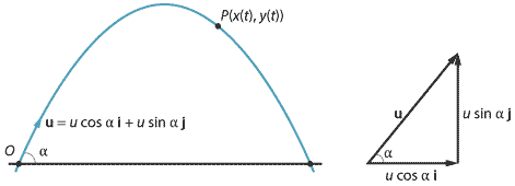

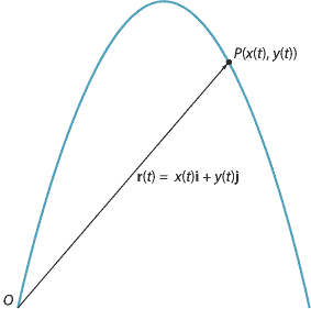
Denote the position vector of the particle at time \(t\), with respect to an origin \(O\), by

\[ \mathbf{r}(t) = x(t)\,\mathbf{i} + y(t)\,\mathbf{j}. \]

Here \(x(t)\) is a function of \(t\) describing the position of the particle in the \(\mathbf{i}\)-direction, and \(y(t)\) is a function of \(t\) describing the position of the particle in the \(\mathbf{j}\)-direction. Assume the particle starts its motion from the origin.

The velocity vector of the particle at time \(t\) is given by

\[ \dot{\mathbf r}(t) = \dot{x}(t)\,\mathbf{i} + \dot{y}(t)\,\mathbf{j}. \]

Here \(\dot{x}(t)\) is the velocity of the particle in the \(\mathbf{i}\)-direction, and \(\dot{y}(t)\) the velocity of the particle in the \(\mathbf{j}\)-direction.

The acceleration vector of the particle at time \(t\) is given by

\[ \ddot{\mathbf r}(t) = \ddot{x}(t)\,\mathbf{i} + \ddot{y}(t)\,\mathbf{j}. \]

We start off as we did for motion in a straight line. Since the acceleration is due to gravity, we have

\[ \ddot{\mathbf r}(t) = -g\,\mathbf{j}. \]

Integrating once gives

\[ \dot{\mathbf r}(t) = -gt\,\mathbf{j} + \mathbf{c}_1, \]

where \(\mathbf{c}_1\) is a vector constant. We are assuming that the initial velocity vector \(\dot{\mathbf r}(0)\) is equal to \(\mathbf{u} = u\cos\alpha\,\mathbf{i} + u\sin\alpha\,\mathbf{j}\), and hence

\[ \dot{\mathbf r}(t) = u\cos\alpha\,\mathbf{i} + (u\sin\alpha - gt)\,\mathbf{j}. \]

Integrating again with respect to \(t\) gives

\[ \mathbf{r}(t) = ut\cos\alpha\,\mathbf{i} + \bigl(ut\sin\alpha - \dfrac{1}{2}gt^2\bigr)\,\mathbf{j} + \mathbf{c}_2, \]

where \(\mathbf{c}_2\) is a vector constant. Since we are assuming that the particle starts at the origin, we have \(\mathbf{r}(0) = \mathbf{0}\) and so \(\mathbf{c}_2 = \mathbf{0}\). Hence,

\[ \mathbf{r}(t) = ut\cos\alpha\,\mathbf{i} + \bigl(ut\sin\alpha - \dfrac{1}{2}gt^2\bigr)\,\mathbf{j}. \]

Since \(y(t)\) can be written as a quadratic function of \(x(t)\), the path of the projectile is a parabola.

These ideas can easily be extended to three dimensions.

Vector calculus was developed by J. Willard Gibbs and Oliver Heaviside near the end of the 19th century, and most of the standard notation and terminology was established by Gibbs and Edwin Bidwell Wilson in their 1901 book Vector analysis . This book is now available free online.

Next page - History and applications - Kinematics before Newton