Content
Integral calculus and motion in a straight line
We can move from the acceleration function to the velocity function and from the velocity function to the position function through integration. Integrating a function always introduces an arbitrary constant. Hence, one or more boundary conditions are required to determine the motion completely.
Example
A particle moves in a straight line. It is initially at rest at the origin. The acceleration of the particle is given by \(\ddot{x}(t) = \dfrac{1}{3}\cos 3t\).
- Find the velocity at time \(t\).
- Find the position at time \(t\).
- Sketch the position–time graph for \(t\in [0,2\pi]\).
Solution
- Starting from \(\ddot{x}(t) = \dfrac{1}{3}\cos 3t\) and integrating once, we obtain \[ \dot{x}(t) = \dfrac{1}{9}\sin 3t + c_1. \] Since \(\dot{x}(0) = 0\), we have \(c_1 = 0\). Hence, \[ \dot{x}(t) = \dfrac{1}{9}\sin 3t. \]
- Integrating again gives \[ x(t) = -\dfrac{1}{27}\cos 3t + c_2. \] Since \(x(0) = 0\), we have \(c_2 = \dfrac{1}{27}\). Hence, \[ x(t) = -\dfrac{1}{27} \cos 3t + \dfrac{1}{27}. \]
-
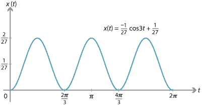
Note. We have \(\ddot{x}(t) = -9x(t) + \dfrac{1}{3}\). Motion that satisfies a differential equation of this form is called simple harmonic motion. The particle oscillates along a straight line between 0 and \(\dfrac{2}{27}\). The centre of the oscillation is at \(x=\dfrac{1}{27}\).
It is often convenient to use calculus to solve problems of motion in a straight line, particularly when the boundary conditions vary. In addition, calculus is often used when we are considering the motion of two or more particles with different starting times and initial positions.
Example
Two particles \(A\) and \(B\) are moving to the right along a straight line. For particle \(A\), we have \(\ddot{x}_A(t) = \dfrac{1}{2}\), with boundary conditions \(x_A(0) = \dfrac{1}{4}\) and \(\dot{x}_A(0) = \dfrac{1}{2}\). For particle \(B\), we have \(\ddot{x}_B(t) = \dfrac{2}{3}\), with boundary conditions \(x_B(1) = \dfrac{1}{2}\) and \(\dot{x}_B(1) = \dfrac{5}{6}\).- Find when and where the two particles have the same position.
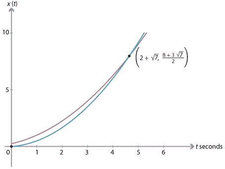
- Sketch the position–time graphs for \(A\) and \(B\) on the one set of axes.
Solution
- Particle \(A\). Starting from \(\ddot{x}_A(t) = \dfrac{1}{2}\) and integrating once, we obtain \(\dot{x}_A(t) = \dfrac{1}{2}t + c_1\). Since \(\dot{x}_A(0) = \dfrac{1}{2}\), we have \(c_1 = \dfrac{1}{2}\), and so \[ \dot{x}_A(t) = \dfrac{1}{2}t + \dfrac{1}{2}. \] Integrating again gives \[ x_A(t) = \dfrac{1}{4} t^2 + \dfrac{1}{2} t + c_2. \] Since \(x_A(0) = \dfrac{1}{4}\), we have \(c_2 = \dfrac{1}{4}\). Hence, \[ x_A(t) = \dfrac{1}{4}\bigl(t^2 + 2t + 1\bigr). \] Particle \(B\). Integrating \(\ddot{x}_B(t) = \dfrac{2}{3}\), we obtain \(\dot{x}_B(t) = \dfrac{2}{3}t + c_3\). Since \(\dot{x}_B(1)=\dfrac{5}{6}\), we have \(c_3 = \dfrac{1}{6}\) and so \[ \dot{x}_B(t) = \dfrac{1}{6}\bigl(4t + 1\bigr). \] Integrating again: \[ x_B(t) = \dfrac{1}{6}\bigl(2t^2 + t\bigr) + c_4. \] Since \(x_B(1) = \dfrac{1}{2}\), we have \(c_4 = 0\) and so \[ x_B(t) = \dfrac{1}{6}\bigl(2t^2 + t\bigr). \] Particles meet. The particles meet when \(x_A(t) = x_B(t)\): \begin{align*} \dfrac{1}{4}\bigl(t^2 + 2t + 1\bigr) &= \dfrac{1}{6}\bigl(2t^2 + t\bigr) \\ t^2 - 4t - 3 &= 0 \\ t &= 2 \pm \sqrt{7}. \end{align*} Since \(t \geq 0\), the particles meet when \(t = 2 + \sqrt{7}\). Substituting in \(x_B(t) = \dfrac{1}{6}(2t^2 + t)\), we have \[ x_B(2 + \sqrt{7}) = \dfrac{1}{6}\bigl(2(2+\sqrt{7})^2 + (2+\sqrt{7})\bigr) = \dfrac{1}{2}\bigl(8 + 3\sqrt{7}\bigr). \] The particles meet at \(\bigl(2+\sqrt{7}, \dfrac{1}{2}(8 + 3\sqrt{7})\bigr)\).
-
Exercise 9
Two particles \(A\) and \(B\) are moving in a straight line. The positions of the particles, with respect to an origin, are given by \(x_A(t) = \dfrac{1}{2}t^2 - t + 3\) and \(x_B(t) = -\dfrac{1}{4}t^2 + t + 1\) at time \(t \geq 0\).
- Prove that \(A\) and \(B\) do not collide.
- How close do \(A\) and \(B\) get to one another?
- During which intervals of time are they moving in opposite directions?
Revisiting the constant-acceleration formulas
We can use calculus to derive the five equations of motion from the section Constant acceleration.
We assume that \(\ddot{x}(t) = a\), where \(a\) is a constant, and that \(x(0) = 0\) and \({\dot{x}(0) = u}\). Integrating \(\ddot{x}(t) = a\) with respect to \(t\) for the first time gives
\[ v(t) = \dot{x}(t) = at + c_1. \]Since \(v(0) = \dot{x}(0) = u\), we have \(c_1 = u\). Hence, we obtain the first equation of motion:
\[ v(t) = u + at. \] Integrating again gives \[ x(t) = ut + \dfrac{1}{2}at^2 + c_2. \] Since \(x(0) = 0\), we have \(c_2 = 0\). This yields the third equation of motion: \[ x(t) = ut + \dfrac{1}{2}at^2. \]The other equations of motion can easily be derived from these two using only algebra.
Using definite integrals to find displacement and change in velocity
The displacement (that is, the change in position) over some time interval can be found directly using a definite integral of the velocity.
If we are given the velocity \(v(t)\) as a function of time, then from \(t = t_1\) to \(t = t_2\), the displacement is given by
\[ \text{Displacement} = \int_{t_1}^{t_2} v(t)\,dt. \]If we are given the acceleration \(\ddot x(t)\) as a function of time, then from \(t = t_1\) to \(t = t_2\), the change in velocity is given by
\[ \text{Change in velocity} = \int_{t_1}^{t_2} \ddot x(t)\,dt. \]Example
A particle is moving with constant acceleration of 5 m/s\(^2\). When \(t = 0\), the velocity of the particle is 4 m/s. Find the displacement of the particle from \(t = 4\) to \(t = 8\).
Solution
The velocity is given by \(v(t) = 4+5t\). Thus, the displacement of the particle from \(t = 4\) to \(t = 8\) is
\[ \int_{4}^{8} (4 + 5t)\,dt = \Biggl[4t + \dfrac{5t^2}{2}\Biggr]_4^8 = 136 \text{ m}. \]Exercise 10
A particle is moving with velocity \(v(t) = \cos(2\pi t)\) at time \(t\). Find the displacement of the particle from
- \(t = 0\) to \(t = \dfrac{1}{4}\)
- \(t = \dfrac{1}{4}\) to \(t = 1\)
- \(t = \dfrac{3}{4}\) to \(t = \dfrac{5}{4}\).
Next page - Links forward - Simple harmonic motion
| This publication is funded by the Australian Government Department of Education, Employment and Workplace Relations |
Contributors Term of use |