Content

Constant velocity

The rate of change of the position of a particle with respect to time is called the velocity of the particle. Velocity is a vector quantity, with magnitude and direction. The speed of a particle is the magnitude of its velocity.

Students have learnt in earlier years that, for motion at a constant speed,

\[ \text{Speed} = \dfrac{\text{Distance travelled}}{\text{Time taken}}. \]

Similarly, for motion at a constant velocity, we have

\[ \text{Velocity} = \dfrac{\text{Displacement}}{\text{Time taken}}. \]

For example, consider a particle which starts at the origin \(O\), moves to a point \(B\) at a constant velocity, and then moves to a point \(A\) at a different constant velocity, as shown in the following diagram.

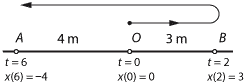
• The particle moves from \(O\) to \(B\) in two seconds. During this time, it has a constant velocity of \(\dfrac{3}{2} = 1.5\) metres per second.
• The particle moves from \(B\) to \(A\) in four seconds. During this time, it has a constant velocity of \(-\dfrac{7}{4} = -1.75\) metres per second.

In this module, we abbreviate 'metres per second' as m/s. The alternative abbreviation ms\(^{-1}\) is also very common.

• If a particle is moving with a constant velocity of 10 m/s, then its displacement over 5 seconds is 50 metres.
• If a particle is moving with a constant velocity of \(-10\) m/s, then its displacement over 5 seconds is \(-50\) metres. The distance travelled is 50 metres.

If a particle is moving with constant velocity, it does not change direction. If the particle is moving to the right, it has positive velocity, and if the particle is moving to the left, it has negative velocity. In general, if a particle is moving at a constant velocity (rate), then its constant velocity \(v\) is determined by the formula

\[ v = \dfrac{x(t_2)-x(t_1)}{t_2-t_1}, \]

where \(x(t_i)\) is the position at time \(t_i\).

There are two important graphical representations for constant velocity. The first is the graph of velocity against time. The second is the graph of position against time.

Velocity–time graphs

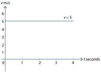
The following diagram shows the velocity–time graph for a particle moving at 5 m/s for 4 seconds. The constant velocity is plotted against time. Naturally, it gives a line segment parallel to the \(t\)-axis. The gradient of this line is zero.

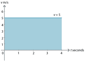
The region between the line segment and the \(t\)-axis is shaded in the following diagram. This region is a rectangle of area \(5 \times 4 = 20\), which is the product of the velocity and the time taken. So this area represents the displacement. The area between the line segment and the \(t\)-axis is the displacement of the particle from \(t=0\) to \(t=4\).

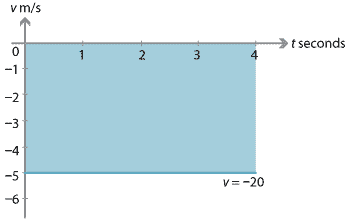
If the particle has a constant velocity of \(-5\) m/s for 4 seconds, as shown in the following diagram, then the region lies below the \(t\)-axis and represents a displacement of \(-20\) m. The region has a signed area of \(-20\). The notion of signed area is introduced in the module Integration.

Finding the displacement of a particle from the velocity–time graph using integration will be discussed in a later section of this module.

Position–time graphs

We can also plot a graph of position against time. In this case, it is the gradient of the graph that is of interest.

Positive velocity

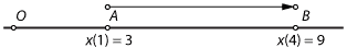
Assume that a particle moves with constant velocity from point \(A\) to point \(B\), as shown in the following diagram. At time \(t = 1\), the position of the particle is 3 m to the right of \(O\), that is, \(x(1) = 3\). At time \(t = 4\), its position is 9 m to the right of \(O\), that is, \(x(4) = 9\).

The displacement (change of position) of the particle is 6 metres over the time interval \([1,4]\). The duration of the motion is 3 seconds. Therefore the constant velocity is 2 m/s. The position–time graph for this motion is as follows.

The gradient of this line is \[ \dfrac{x(4)-x(1)}{4-1} = \dfrac{9-3}{4-1} = \dfrac{6}{3} = 2. \]

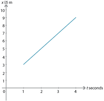
Since this is the displacement divided by the time taken, the gradient of the line is equal to the velocity. It is always the case that, for a particle moving with constant velocity, the gradient of the position–time graph gives the velocity of the particle.

Negative velocity

Assume that a particle moves with constant velocity from \(A\) to \(B\), as in the following diagram. At time \(t = 1\), the position of the particle is 3 m to the right of \(O\), that is, \(x(1) = 3\). At time \(t = 4\), its position is 3 m to the left of \(O\), that is, \(x(4) = -3\).

The displacement is \(-6\) metres over 3 seconds. Therefore the constant velocity is \(-2\) m/s. The gradient of the position–time graph, shown below, is

\[ \dfrac{x(4)-x(1)}{4-1} = \dfrac{-3-3}{4-1} = \dfrac{-6}{3} = -2. \]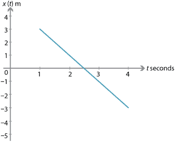

Throughout this module, we often use the gradient of a position–time graph to determine velocity, and use the area under a velocity–time graph to determine displacement. These are both important ideas, which will be further developed using calculus.

Next page - Content - Constant acceleration