Links forward

Striking it lucky with \(e\)

You're digging for gold on the goldfields. It's a plentiful gold field, and every time you dig, you obtain an amount of gold between 0 and 1 gram. The amount of gold you find each time is random and uniformly distributed. How many times do you expect to have to dig before you obtain a total of 1 gram of gold?

You might think that the answer is twice! Actually, the expected number of digs is \(e\).

To put the question in pure mathematical terms, the amount of gold (in grams) you obtain each time you dig is a random variable uniformly distributed in \([0,1]\). Let \(X_1\) be the amount you obtain the first time you dig, let \(X_2\) be the amount the second time you dig and, in general, let \(X_n\) be the amount of gold found the \(n\)th time you dig. So each \(X_n\) is a random variable uniformly distributed in \([0,1]\).

The number of times you have to dig to obtain 1 gram is then the least \(n\) such that \({X_1 + X_2 + \dotsb + X_n \geq 1}\). Let this number be \(M\). It is also a random variable:

\[ M = \min \bigl\{\, n : X_1 + X_2 + \dotsb + X_n \geq 1 \,\bigr\}. \]

The number of times you expect to have to dig to obtain 1 gram of gold is the expected value \(E(M)\) of \(M\).

The probability that you obtain a full gram in your first dig is zero — you have to get a whole gram, and the chances of that are vanishingly small: \(\Pr(M=1)=0\).

The probability you obtain a gram in two digs is \(\dfrac{1}{2}\): you could get anywhere from 0 to 2 grams, and 1 is right in the middle.

In general, the probability that you obtain a gram on the \(n\)th dig, but not earlier, can be expressed as follows. It's the probability that you have less than a gram after \(n-1\) digs, but are not still below a gram after \(n\) digs:

\begin{align*} \Pr(M = n) &= \Pr(X_1 + \dotsb + X_{n-1} < 1 \text{ and } X_1 + \dotsb + X_n \geq 1) \\ &= \Pr(X_1 + \dotsb + X_{n-1} < 1) - \Pr(X_1 + \dotsb + X_n < 1). \end{align*}

As it turns out,⁴ the probability that you have less than a gram after \(n\) digs is

\[ \Pr (X_1 + \dotsb + X_n < 1) = \dfrac{1}{n!}. \]

Proving this requires some work with integration and probability distribution functions.

From this, we obtain

\[ \Pr(M=n) = \dfrac{1}{(n-1)!} - \dfrac{1}{n!}. \]

Thus \(\Pr(M=1) = 0\) and, for \(n>1\), we can simplify to

\begin{align*} \Pr(M=n) &= \dfrac{1}{(n-1)!} \Bigl( 1 - \dfrac{1}{n} \Bigr)\\ &= \dfrac{1}{(n-1)!} \cdot \dfrac{n-1}{n}\\ &= \dfrac{1}{n} \cdot \dfrac{1}{(n-2)!}. \end{align*}

Knowing this probability, we see that the expected number of digs required is

\begin{align*} E(M) &= 1 \Pr(M=1) + 2 \Pr(M=2) + 3 \Pr (M=3) + 4 \Pr (M=4) + \dotsb \\ &= 1 \cdot 0 + 2 \cdot \dfrac{1}{2} \cdot \dfrac{1}{0!} + 3 \cdot \dfrac{1}{3} \cdot \dfrac{1}{1!} + 4 \cdot \dfrac{1}{4} \cdot \dfrac{1}{2!} + \dotsb \\ &= 1 + \dfrac{1}{1!} + \dfrac{1}{2!} + \dfrac{1}{3!} + \dotsb = e. \end{align*}

We have yet to hear of any goldfields with such a distribution of gold.

Sandwiching \(e\)

By considering the integral

\[ \int_n^{n+1} \dfrac{1}{x} \; dx, \] where \(n\) is positive, we will obtain another amazing formula for \(e\).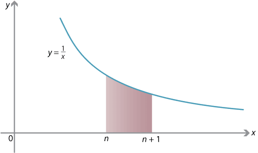

Detailed description

On the one hand, we can compute the integral exactly:

\begin{align*} \int_n^{n+1} \dfrac{1}{x} \; dx &= \bigl[ \ln x \bigr]_n^{n+1}\\ &= \ln (n+1) - \ln n\\ &= \ln \dfrac{n+1}{n}\\ &= \ln \Bigl( 1 + \dfrac{1}{n} \Bigr). \end{align*}

On the other hand, on the interval \([n,n+1]\), we see that the function \(\smash{\dfrac{1}{x}}\) satisfies

\[ \dfrac{1}{n+1} \leq \dfrac{1}{x} \leq \dfrac{1}{n}. \]

Using these inequalities to estimate the integral (see the module Integration for details), we have

\[ \dfrac{1}{n+1} \leq \int_n^{n+1} \dfrac{1}{x} \; dx = \ln \Bigl( 1 + \dfrac{1}{n} \Bigr) \leq \dfrac{1}{n}. \]

Multiplying through by \(n\) and using a logarithm law gives

\[ \dfrac{n}{n+1} \leq n \, \ln \Bigl( 1 + \dfrac{1}{n} \Bigr) = \ln \Bigl(1 + \dfrac{1}{n}\Bigr)^n \leq 1. \]

The expression \(\ln (1 + \dfrac{1}{n})^n\) is sandwiched between \(\dfrac{n}{n+1}\) and 1. In fact, as \(n \to \infty\), \(\dfrac{n}{n+1} \to 1\) as well, and so we can deduce

\[ \lim_{n \to \infty} \ln \Bigl( 1 + \dfrac{1}{n} \Bigr)^n = 1. \]

It follows that the limit of \((1+\dfrac{1}{n})^n\), as \(n \to \infty\), is a number whose natural logarithm is 1, that is, \(e\). We have our new formula for \(e\):

\[ \lim_{n \to \infty} \Bigl( 1 + \dfrac{1}{n} \Bigr)^n = e. \]

Next page - History and applications