Appendix

Exactness of area estimates

Consider some simple functions \(f(x)\) — constant, linear, quadratic — and see how the various estimates fare in approximating the integral \(\int_a^b f(x) \; dx\).

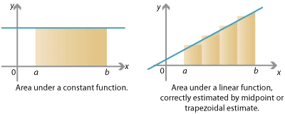
First suppose \(f(x)\) is a constant function. In this case, we obtain an exactly correct answer for the area under the graph from the left-endpoint, right-endpoint, midpoint or trapezoidal estimate. The area under \(y=f(x)\) is itself a rectangle; breaking it up into rectangles or trapezia, we still have the exactly correct area. This is true regardless of the number of subintervals \(n\): we could split \([a,b]\) into just one subinterval, or a million; in all cases we obtain the exactly correct answer.

Detailed description of diagrams

Next suppose \(f(x)\) is a (non-constant) linear function. In this case the left- and right- endpoint estimates will definitely not give you the correct answer. However, the midpoint and trapezoidal estimates will give you the exactly correct answer. The midpoint estimate builds rectangles which have exactly the same amount of area above and below the line. And breaking the area under \(y=f(x)\) into trapezia gives the exactly correct area. Again this is true whatever number of subintervals we take.

However, when \(f(x)\) is a quadratic function, in general none of the left-endpoint, right-endpoint, midpoint or trapezoidal estimates will give the correct area. Let's consider the function \(f(x) = x^2\), and see how the midpoint and trapezoidal estimates fare. We'll just take one subinterval, \(n=1\), so \(\Delta x = b-a\).

First, the midpoint estimate \(M\) is just

\[ M = f \Big( \frac{a+b}{2} \Big) \; \Delta x = \Big( \frac{1}{4} a^2 + \frac{1}{2} ab + \frac{1}{4} b^2 \Big) \, \big( b-a \big). \]

Next, the trapezoidal estimate \(T\) (again with only one subinterval) is

\[ T = \Big( \frac{1}{2} f(a) + \frac{1}{2} f(b) \Big) \; \Delta x = \Big( \frac{1}{2} a^2 + \frac{1}{2} b^2 \Big) \, \big( b-a \big). \]

The correct answer, on the other hand, is

\[ \int_a^b x^2 \; dx = \Bigg[ \frac{x^3}{3} \Bigg]_a^b = \frac{1}{3} b^3 - \frac{1}{3} a^3 = \frac{1}{3} \big( a^2 + ab + b^2 \big) \, \big( b-a \big). \]

Here we used the factorisation \(b^3 - a^3 = (b-a)(a^2 + ab + b^2)\).

Note that \(M\) and \(T\) contain very similar terms to the correct answer. Indeed, we can combine the midpoint and trapezoidal estimates to get the exact answer! Observe that

\[ \frac{1}{3} \big(2M + T\big) = \frac{1}{3} \big(b-a\big) \big(a^2 + ab + b^2\big) = \int_a^b x^2 \; dx. \]

This combination of the midpoint and trapezoidal rules will in fact give us an exactly correct answer for the integral of any quadratic function.

This new area estimate is nothing other than Simpson's rule. Writing out \(\frac{1}{3}(2M+T)\) for a general function \(f(x)\), from the definitions of the midpoint and trapezoidal rules, we have

\begin{align*} \frac{2}{3} M + \frac{1}{3} T &= \big(b-a\big) \; \Bigg( \frac{1}{6} f(a) + \frac{2}{3} f \Big( \frac{a+b}{2} \Big) + \frac{1}{6} f(b) \Bigg) \\ &= \frac{b-a}{2} \; \Bigg( \frac{1}{3} f(a) + \frac{4}{3} f \Big( \frac{a+b}{2} \Big) + \frac{1}{3} f(b) \Bigg). \end{align*}

This pattern of coefficients \(\frac{1}{3}\), \(\frac{4}{3}\), \(\frac{1}{3}\) is exactly Simpson's rule with two subintervals; if we take \(\frac{1}{3}(2M+T)\) for the midpoint and trapezoidal estimates with \(n\) subintervals, we obtain Simpson's rule with \(2n\) subintervals.

Simpson's rule is very accurate because it gets quadratic integrals exactly right. It does this by taking the midpoint and trapezoidal estimates — the previous best estimates, giving exactly correct answers for linear integrals — and combining them. We can also think of Simpson's rule as approximating a function by parabolic segments and computing the integrals of the parabolic segments. It turns out that Simpson's rule actually gets cubic integrals exactly right as well!

Next page - Appendix - Functions integrable and not