Content

Velocity–time graphs

Let us now return to our original motivating question with the bike and speedometer. Let \(v(t)\) denote your velocity on your bike at time \(t\), and we now calculate your total change in position between time \(t=a\) and \(t=b\). As mentioned earlier, if \(v(t)\) is a constant function, and so you are travelling at constant velocity, then your total change in position, or displacement, is \(\Delta s = v \; \Delta t\).

Our idea of estimating your distance travelled by breaking your trip up into 1-minute intervals is nothing more than an area estimate. We may divide the time interval \([a,b]\) into \(n\) subintervals \([t_0, t_1], [t_1, t_2], \dots, [t_{n-1}, t_n]\), each of width \(\Delta t = \frac{1}{n} (b-a)\). We can estimate your velocity over the interval \([t_{j-1}, t_j]\) by the constant \(v(t_j)\) (i.e., using the right-endpoint estimate); over this interval of time, you travelled a distance of approximately \(v(t_j) \; \Delta t\). The total distance travelled, then, is approximately

\[ \sum_{j=1}^n v(t_j) \; \Delta t. \]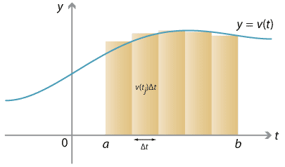

Detailed description of diagram

\[\text{The right-endpoint estimate for area under} \ y = v(t) \ \text{estimates displacement.}\]

In the limit, as we take more and more shorter and shorter time intervals, we obtain the exact change in position (displacement) as,

\[ \int_a^b v(t) \; dt. \]

Therefore, the total displacement is the area under the velocity–time graph \(y = v(t)\).

Note that this integrand is expressed as a function of \(t\), and \(dt\) indicates that we integrate over~\(t\). If we used \(v(x)\) and \(dx\) instead, the meaning would be identical:

\[ \int_a^b v(t) \; dt = \int_a^b v(x) \; dx. \]

The variable \(t\) (or \(x\)) just indexes the values of the integrand; it is only used for the integral's own bookkeeping purposes. It is known as a dummy variable, analogous to the dummy variable in summation notation, like the \(j\) in \(\sum_{j=1}^5 j^2\).

Next page - Content - Areas above and below the axis