History and applications
History
The history of calculus is discussed in the modules:Applications
Application in biology
Example: Chemotherapy
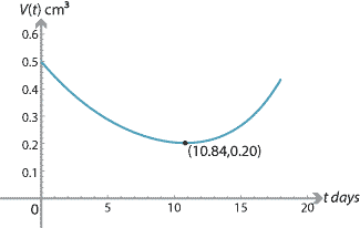
Malignant tumours respond to radiation therapy and chemotherapy. Consider a medical experiment in which mice with tumours are given a chemotherapeutic drug. At the time of the drug being administered, the average tumour size is about 0.5 cm\(^3\). The tumour volume \(V(t)\) after \(t\) days is modelled by
\[ V(t) = 0.005e^{0.24t} + 0.495e^{-0.12t}, \]for \(0\leq t \leq 18\). Let us find the minimum point. The first and second derivatives are
\begin{align*} V'(t) &= 0.0012e^{0.24t} - 0.0594e^{-0.12t} \\ V''(t) &= 0.000288e^{0.24t} + 0.007128e^{-0.12t}. \end{align*}Note that \(V''(t) > 0\), for all \(t\) in the domain. By solving \(V'(t) = 0\), we find that the minimum point occurs when \(t \approx 10.84\) days. The volume of the tumour is approximately 0.20 cm\(^3\) at this time.
Applications in physics
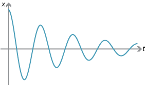
Calculus is essential in many areas of physics. Some additional applications of calculus to physics are given in the modules Motion in a straight line and The calculus of trigonometric functions.Example: Damped simple harmonic motion
The displacement of a body of mass \(m\) undergoing damped harmonic motion is given by the formula
\[ x = Ae^{-\frac{bt}{2m}}\cos(\omega t), \]where
\[ \omega = \sqrt{\dfrac{k}{m}-\Bigl(\dfrac{b}{2m}\Bigr)^2}. \]Here \(k\) and \(b\) are positive constants. (Note that damped simple harmonic motion reduces to simple harmonic motion when \(b=0\).)
The motion can be investigated by using calculus to find the turning points.
Since \(x = Ae^{-\frac{bt}{2m}}\cos(\omega t)\), we have \begin{align*} \dfrac{dx}{dt} &= -\dfrac{b}{2m}Ae^{-\frac{bt}{2m}}\cos(\omega t) - A\omega e^{-\frac{bt}{2m}}\sin(\omega t) \\ &= -Ae^{-\frac{bt}{2m}}\Bigl(\dfrac{b}{2m}\cos(\omega t) + \omega\sin(\omega t)\Bigr). \end{align*} The stationary points are found by putting \(\dfrac{dx}{dt} = 0\). This implies \[ \tan(\omega t) = -\dfrac{b}{2m\omega}. \]Here is example from optics using related rates of change.
Example: Thin lens formula
The thin lens formula in physics is
\[ \dfrac{1}{s} + \dfrac{1}{S} = \dfrac{1}{f}, \]where \(s\) is the distance of an object from the lens, \(S\) is the distance of the image from the lens, and \(f\) is the focal length of the lens. Here \(f\) is a constant, and \(s\) and \(S\) are variables.
Suppose the object is moving away from the lens at a rate of 3 cm/s. How fast and in which direction will the image be moving?
We are given \(\dfrac{ds}{dt} = 3\). The question is: What is \(\dfrac{dS}{dt}\)?
We know by the chain rule that
\[ \dfrac{dS}{dt} = \dfrac{dS}{ds} \times \dfrac{ds}{dt} = \dfrac{dS}{ds} \times 3. \]
Making \(S\) the subject of the thin lens formula, we have \(S = \dfrac{fs}{s-f}\). The derivative of \(S\) with respect to \(s\) is
\[ \dfrac{dS}{ds} = \dfrac{-f^2}{(s-f)^2}. \]Thus
\[ \dfrac{dS}{dt} = \dfrac{-f^2}{(s-f)^2} \times 3 = \dfrac{-3f^2}{(s-f)^2}. \]The image is moving towards the lens at \(\dfrac{3f^2}{(s-f)^2}\) cm/s.
Next page - Answers to exercises
| This publication is funded by the Australian Government Department of Education, Employment and Workplace Relations |
Contributors Term of use |