Content
Graph sketching
Increasing and decreasing functions
Let \(f\) be some function defined on an interval.
Definition
The function \(f\) is increasing over this interval if, for all points \(x_1\) and \(x_2\) in the interval,
\[ x_1 \leq x_2 \ \implies\ f(x_1) \leq f(x_2). \]This means that the value of the function at a larger number is greater than or equal to the value of the function at a smaller number.
The graph on the left shows a differentiable function. The graph on the right shows a piecewise-defined continuous function. Both these functions are increasing.
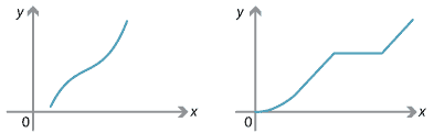
Examples of increasing functions.
Definition
The function \(f\) is decreasing over this interval if, for all points \(x_1\) and \(x_2\) in the interval,
\[ x_1 \leq x_2 \ \implies\ f(x_1)\geq f(x_2). \]The following graph shows an example of a decreasing function.
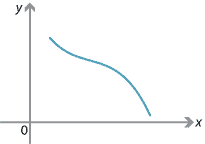
Example of a decreasing function.
Note that a function that is constant on the interval is both increasing and decreasing over this interval. If we want to exclude such cases, then we omit the equality component in our definition, and we add the word strictly:
- A function is strictly increasing if \(x_1<x_2\) implies \(f(x_1)<f(x_2)\).
- A function is strictly decreasing if \(x_1<x_2\) implies \(f(x_1)>f(x_2)\).
We will use the following results. These results refer to intervals where the function is differentiable. Issues such as endpoints have to be treated separately.
- If \(f'(x) > 0\) for all \(x\) in the interval, then the function \(f\) is strictly increasing.
- If \(f'(x) < 0\) for all \(x\) in the interval, then the function \(f\) is strictly decreasing.
- If \(f'(x) = 0\) for all \(x\) in the interval, then the function \(f\) is constant.
Stationary points
Definitions
Let \(f\) be a differentiable function.
- A stationary point of \(f\) is a number \(x\) such that \(f'(x) = 0\).
- The point \(c\) is a maximum point of the function \(f\) if and only if \(f(c)\geq f(x)\), for all \(x\) in the domain of \(f\). The value \(f(c)\) of the function at \(c\) is called the maximum value of the function.
- The point \(c\) is a minimum point of the function \(f\) if and only if \(f(c)\leq f(x)\), for all \(x\) in the domain of \(f\). The value \(f(c)\) of the function at \(c\) is called the minimum value of the function.
Local maxima and minima
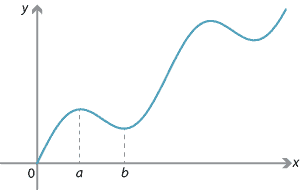
In the following diagram, the point \(a\) looks like a maximum provided we stay close to it, and the point \(b\) looks like a minimum provided we stay close to it.
Definitions
- The point \(c\) is a local maximum point of the function \(f\) if there exists an interval \((a,b)\) with \(c\in (a,b)\) such that \(f(c) \geq f(x)\), for all \(x\in (a,b)\).
- The point \(c\) is a local minimum point of the function \(f\) if there exists an interval \((a,b)\) with \(c\in (a,b)\) such that \(f(c) \leq f(x)\), for all \(x\in (a,b)\).
These are sometimes called relative maximum and relative minimum points. Local maxima and minima are often referred to as turning points.
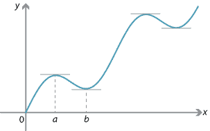
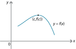
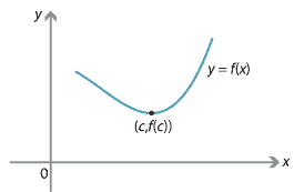
The following diagram shows the graph of \(y=f(x)\), where \(f\) is a differentiable function. It appears from the diagram that the tangents to the graph at the points which are local maxima or minima are horizontal. That is, at a local maximum or minimum point \(c\), we have \(f'(c) = 0\), and hence each local maximum or minimum point is a stationary point.
The result appears graphically obvious, but we will present a formal proof in the case of a local maximum.
Theorem
Let \(f\) be a differentiable function. If \(c\) is a local maximum point, then \(f'(c) = 0\).
Proof
Consider the interval \((c-\delta,c+\delta)\), with \(\delta > 0\) chosen so that \(f(c) \geq f(x)\) for all \(x \in (c-\delta,c+\delta)\).
For all positive \(h\) such that \(0 < h < \delta\), we have \(f(c) \geq f(c+h)\) and therefore
\[ \dfrac{f(c+h) - f(c)}{h} \leq 0. \]Hence,
\[ f'(c) = \lim_{h \to 0^+} \dfrac{f(c+h) - f(c)}{h} \leq 0. \qquad (1) \]For all negative \(h\) such that \(-\delta < h < 0\), we have \(f(c) \geq f(c+h)\) and therefore
\[ \dfrac{f(c+h) - f(c)}{h} \geq 0. \]Hence,
\[ f'(c) = \lim_{h \to 0^-} \dfrac{f(c+h) - f(c)}{h} \geq 0. \qquad (2) \]From (1) and (2), it follows that \(f'(c) = 0\).
\(\Box\)
The first derivative test for local maxima and minima
The derivative of the function can be used to determine when a local maximum or local minimum occurs.
Theorem (First derivative test)
Let \(f\) be a differentiable function. Suppose that \(c\) is a stationary point, that is, \(f'(c) = 0\).
- If there exists \(\delta > 0\) such that \(f'(x) > 0\), for all \(x \in (c-\delta,c)\), and \(f'(x) < 0\), for all \(x \in (c,c+\delta)\), then \(c\) is a local maximum point.
- If there exists \(\delta > 0\) such that \(f'(x) < 0\), for all \(x \in (c-\delta,c)\), and \(f'(x) > 0\), for all \(x \in (c,c+\delta)\), then \(c\) is a local minimum point.
Proof
- The function is increasing on the interval \((c-\delta,c)\), and decreasing on the interval \((c,c+\delta)\). Hence, \(f(c) \geq f(x)\) for all \(x\in (c-\delta,c+\delta)\).
- The function is decreasing on the interval \((c-\delta,c)\), and increasing on the interval \((c,c+\delta)\). Hence, \(f(c) \leq f(x)\) for all \(x\in (c-\delta,c+\delta)\).
\(\Box\)
In simple language, the first derivative test says:
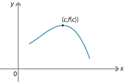
- If \(f'(c) = 0\) with \(f'(x) > 0\) immediately to the left of \(c\) and \(f'(x) < 0\) immediately to the right of \(c\), then \(c\) is a local maximum point.
We can also illustrate this with a gradient diagram.
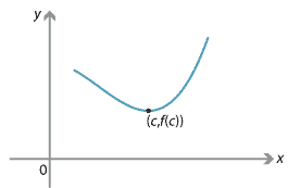
Value of \(x\) \(c\) Sign of \(f'(x)\) + 0 − Slope of graph \(y=f(x)\) \(\diagup\) — \(\diagdown\) - If \(f'(c) = 0\) with \(f'(x) < 0\) immediately to the left of \(c\) and \(f'(x) > 0\) immediately to the right of \(c\), then \(c\) is a local minimum point.
We can also illustrate this with a gradient diagram.
Value of \(x\) \(c\) Sign of \(f'(x)\) + 0 − Slope of graph \(y=f(x)\) \(\diagdown\) — \(\diagup\)
There is another important type of stationary point:
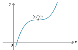
- If \(f'(c) = 0\) with \(f'(x) > 0\) on both sides of \(c\), then \(c\) is a stationary point of inflexion.
Here is a gradient diagram for this situation.
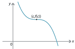
Value of \(x\) \(c\) Sign of \(f'(x)\) + 0 − Slope of graph \(y=f(x)\) \(\diagup\) — \(\diagup\) - If \(f'(c) = 0\) with \(f'(x) < 0\) on both sides of \(c\), then \(c\) is a stationary point of inflexion.
Here is a gradient diagram for this situation.
Value of \(x\) \(c\) Sign of \(f'(x)\) + 0 − Slope of graph \(y=f(x)\) \(\diagdown\) — \(\diagdown\)
Example
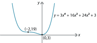
Find the stationary points of \(f(x) = 3x^4+16x^3+24x^2+3\), and determine their nature.
Solution
The derivative of \(f\) is
\begin{align*} f'(x) &= 12x^3+48x^2+48x \\ &= 12x(x^2+4x+4) \\ &= 12x(x+2)^2. \end{align*}So \(f'(x) = 0\) implies \(x=0\) or \(x=-2\).
- If \(x < -2\), then \(f'(x) < 0\).
- If \(-2 < x < 0\), then \(f'(x) < 0\).
- If \(x > 0\), then \(f'(x) > 0\).
We can represent this in a gradient diagram.
| Value of \(x\) | −2 | 0 | |||
|---|---|---|---|---|---|
| Sign of \(f'(x)\) | + | 0 | − | 0 | + |
| Slope of graph \(y=f(x)\) | \(\diagdown\) | — | \(\diagdown\) | — | \(\diagup\) |
Hence, there are stationary points at \(x=0\) and \(x=-2\): there is a local minimum at \(x=0\), and a stationary point of inflexion at \(x=-2\).
The graph of \(y = f(x)\) is shown in the following diagram, but not all the features of the graph have been carefully considered at this stage.
Exercise 1
Assume that the derivative of the function \(f\) is given by \(f'(x) = (x-1)^2(x-3)\). Find the values of \(x\) which are stationary points of \(f\), and state their nature.
Use of the second derivative
The second derivative is introduced in the module Introduction to differential calculus. Using functional notation, the second derivative of the function \(f\) is written as \(f''\). Using Leibniz notation, the second derivative is written as \(\dfrac{d^2 y}{dx^2}\), where \(y\) is a function of \(x\).
In the module Motion in a straight line, it is shown that the acceleration of a particle is the second derivative of its position with respect to time. That is, if the position of the particle at time \(t\) is denoted by \(x(t)\), then the acceleration of the particle is \(\ddot x(t)\).
Recall that, in kinematics, \(\dot x\) means \(\dfrac{dx}{dt}\) and \(\ddot x\) means \(\dfrac{d^2x}{dt^2}\).
Concave up and concave down
Let \(f\) be a function defined on the interval \((a,b)\), and assume that \(f'\) and \(f''\) exist at all points in \((a,b)\). We consider the shape of the curve \(y = f(x)\).
If \(f''(x) > 0\), for all \(x \in (a,b)\), then the slope of the curve is increasing in the interval \((a,b)\). The curve is said to be concave up.
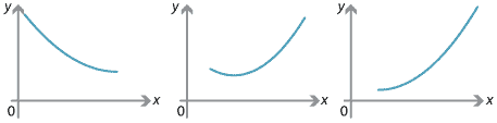
Figure : Examples of concave-up curves.
If \(f''(x) < 0\), for all \(x \in (a,b)\), then the slope of the curve is decreasing in the interval \((a,b)\). The curve is concave down.
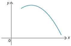
Figure : Example of a concave-down curve.
Inflexion points
A point where the curve changes from concave up to concave down, or from concave down to concave up, is called a point of inflexion. In the following diagram, there are points of inflexion at \(x=c\) and \(x=d\).
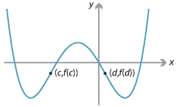
Examples of points of inflexion.
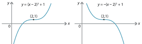
The graphs of \(y=(x-2)^3+1\) and \(y=-(x-2)^3 + 1\) are shown below. The point \((2,1)\) is a point of inflexion for each of these graphs. In fact, the point \((2,1)\) is a stationary point of inflexion for each of these graphs.
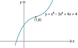
The graph of \(y=x^3-3x^2+4x+4\) is as follows. It has a point of inflexion at \((1,6)\), but this is not a stationary point. In fact, this function has \(\dfrac{dy}{dx} > 0\), for all \(x\).
Note. Clearly, a necessary condition for a twice-differentiable function \(f\) to have a point of inflexion at \(x = c\) is that \(f''(c) = 0\). We will see that this is not a sufficient condition, and care must be taken when using it to find an inflexion point. For there to be a point of inflexion, there must be a change of concavity.
Example
Find the inflexion point of the cubic function \(f(x) = x^3 - 3x^2 - 144x\).
Solution
We find the first and second derivatives:
\[ f'(x) = 3x^2 - 6x - 144 \qquad\text{and}\qquad f''(x) = 6x - 6. \]Thus \(f''(x)=0\) implies \(x=1\). For \(x<1\), we have \(f''(x)<0\). For \(x>1\), we have \(f''(x)>0\). The curve changes from concave down to concave up at \(x=1\). Hence, there is a point of inflexion at \(x=1\).
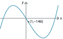
It is not hard to show that there is a local maximum at \(x=-6\) and a local minimum at \(x=8\).
The second derivative test
We have seen how to use the first derivative test to determine whether a stationary point is a local maximum, a local minimum or neither of these. The second derivative provides an alternative test.
Theorem (Second derivative test)
Suppose \(f\) is twice differentiable at a stationary point \(c\).
- If \(f''(c)<0\), then \(f\) has a local maximum at \(c\).
- If \(f''(c)>0\), then \(f\) has a local minimum at \(c\).
We will prove the first part of this theorem. The proof of the second part is similar.
Proof
Assume that \(f''(c)<0\). Then \(f'(x)\) is strictly decreasing over some interval around \(c\). Hence, there is a positive number \(\delta\) such that \(f'(x)\) is strictly decreasing on the interval \((c-\delta,c+\delta)\).
We now use the first derivative test.
- To the left of \(c\): For any \(h\in (c-\delta,c)\), we have \(f'(h) > f'(c) = 0\).
- To the right of \(c\): For any \(k\in (c,c+\delta)\), we have \(f'(k) < f'(c) = 0\).
It follows from the first derivative test that \(c\) is a local maximum point.
\(\Box\)
If \(c\) is a stationary point with \(f''(c) =0\), then we cannot use the second derivative test to determine if it is a local maximum, a local minimum or neither of these.
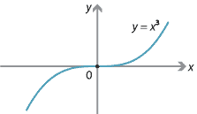
For example, if \(f(x) = x^3\), then \(f'(0) = 0\) and \(f''(0) = 0\). In this case, there is a stationary point of inflexion at 0.
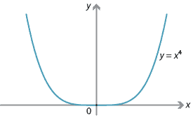
If \(f(x) = x^4\), then \(f'(0) = 0\) and \(f''(0) = 0\). In this case, there is a local minimum at 0.
Thus the second derivative cannot be used as a test when \(f'(c) = f''(c) = 0\).
Example
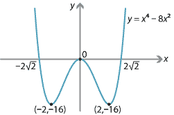
Locate and describe the stationary points of \(f(x) = x^4 - 8x^2\).
Solution
The first derivative is \(f'(x) = 4x^3-16x\), and the second derivative is \(f''(x)= 12x^2-16\). We find the stationary points by solving \(f'(x) = 0\):
\begin{align*} 4x^3-16x &= 0 \\ 4x(x^2-4) &= 0. \end{align*}Hence, the stationary points are at \(x= 0\), \(x = 2\) and \(x=-2\). We use the first derivative test by considering a gradient diagram.
| Value of \(x\) | −2 | 0 | 2 | ||||
|---|---|---|---|---|---|---|---|
| Sign of \(f'(x)\) | − | 0 | + | 0 | − | 0 | + |
| Slope of graph \(y=f(x)\) | \(\diagdown\) | — | \(\diagup\) | — | \(\diagdown\) | — | \(\diagup\) |
- There is a local minimum at \(x=-2\).
- There is a local maximum at \(x=0\).
- There is a local minimum at \(x=2\).
We can also check the local minimum and maximum points using the second derivative test, by considering the values of the second derivative:
- \(f''(-2) = 32 > 0\), so there is a local minimum at \(x=-2\)
- \(f''(0) = -16 < 0\), so there is a local maximum at \(x=0\)
- \(f''(2) = 32 > 0\), so there is a local minimum at \(x=2\).
The question has not required us to sketch the graph. But we have enough information to complete a good sketch if we also observe that the \(x\)-intercepts are \(0\), \(2\sqrt{2}\) and \(-2\sqrt{2}\).
Exercise 4
Locate and describe the stationary points of the graph of \(y=f(x)\) if \(f'(x) =x^3(x^2-5)\).
Next page - Content - More graph sketching
| This publication is funded by the Australian Government Department of Education, Employment and Workplace Relations |
Contributors Term of use |