Motivation

How fast are you really going?

You ride your bicycle down a straight bike path. As you proceed, you keep track of your exact position — so that, at every instant, you know exactly where you are. How fast were you going one second after you started?

This is not a very realistic situation — it's hard to measure your position precisely at every instant! Nonetheless, let us suspend disbelief and imagine you have this information. (Perhaps you have an extremely accurate GPS or a high-speed camera.) By considering this question, we are led to some important mathematical ideas.

First, recall the formula for average velocity:

\[ v = \dfrac{\Delta x}{\Delta t}, \]

where \(\Delta x\) is the change in your position and \(\Delta t\) is the time taken. Thus, average velocity is the rate of change of position with respect to time.

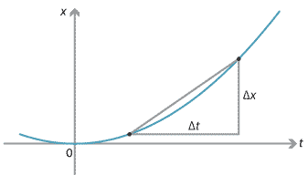
Draw a graph of your position \(x(t)\) at time \(t\) seconds. Connect two points on the graph, representing your position at two different times. The gradient of this line is your average velocity over that time period.

Detailed description
Figure : Average velocity \(v = \dfrac{\Delta x}{\Delta t}\).

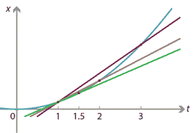
Trying to discover your velocity at the one-second mark (\(t=1\)), you calculate your average velocity over the period from \(t=1\) to a slightly later time \(t = 1 + \Delta t\). Trying to be more accurate, you look at shorter time intervals, with \(\Delta t\) smaller and smaller. If you really knew your position at every single instant of time, then you could work out your average velocity over any time interval, no matter how short. The three lines in the following diagram correspond to \(\Delta t = 2\), \(\Delta t = 1\) and \(\Delta t = 0.5\).

Detailed description
Figure : Average velocity over shorter time intervals.

As \(\Delta t\) approaches 0, you obtain better and better estimates of your instantaneous velocity at the instant \(t=1\). These estimates correspond to the gradients of lines connecting closer and closer points on the graph.

In the limit, as \(\Delta t \to 0\),

\[ \lim_{\Delta t \to 0} \dfrac{\Delta x}{\Delta t} \]

gives the precise value for the instantaneous velocity at \(t=1\). This is also the gradient of the tangent to the graph at \(t=1\). Instantaneous velocity is the instantaneous rate of change of position with respect to time.

Although the scenario is unrealistic, these ideas show how you could answer the question of how fast you were going at \(t=1\). Given a function \(x(t)\) describing your position at time \(t\), you could calculate your exact velocity at time \(t=1\).

In fact, it is possible to calculate the instantaneous velocity at any value of \(t\), obtaining a function which gives your instantaneous velocity at time \(t\). This function is commonly denoted by \(x'(t)\) or \(\dfrac{dx}{dt}\), and is known as the derivative of \(x(t)\) with respect to \(t\).

In this module, we will discuss derivatives.

 

Next page - Motivation and Knowledge - The more things change …