Links forward

Approximating functions

If we are given a function \(f(x)\), we can try to find a polynomial \(p(x)\) which approximates that function. Indeed, if we know some of the values of \(f\),

\[ f(x_1) = y_1, \qquad f(x_2) = y_2, \qquad \dots, \qquad f(x_n) = y_n, \]

then we can find a polynomial \(p(x)\) which takes those values, as we just saw.

That is one type of approximation. The following example shows another type of approximation: finding a polynomial which agrees with \(f\), and its derivatives, at a point.

Example

Find a quadratic polynomial \(p(x)\) which approximates the function \(f(x) = \cos x\) in the sense that \(p\) agrees with \(f\) in value, and in its first two derivatives, at \(x=0\), i.e.,

\[ p(0) = f(0), \qquad p'(0) = f'(0) \qquad \text{and} \qquad p''(0) = f''(0). \]

(Reality check: We're asked to find a quadratic polynomial satisfying three conditions. This makes sense since a quadratic has three coefficients.)

Solution

First of all we can compute \(f'(x) = -\sin x\) and \(f''(x) = -\cos x\), so \(f(0) = 1\), \(f'(0) = 0\) and \(f''(0) = -1\). Thus we want to find a quadratic polynomial \(p(x)\) such that

\[ p(0) = 1, \qquad p'(0) = 0 \qquad \text{and} \qquad p''(0) = -1. \]

Let \(p(x) = ax^2 + bx + c\), where \(a,b,c\) are real coefficients. Then we have \(p'(x) = 2ax + b\) and \(p''(x) = 2a\), so the three equations above become

\[ c = 1, \qquad b = 0 \qquad \text{and} \qquad 2a = -1. \]

Hence \(p(x) = -\frac{1}{2} x^2 + 1\).

We just showed that \(p(x) = 1 - \frac{1}{2} x^2\) is a good approximation to \(f(x) = \cos x\) near \(x=0\). A comparison of the graphs shows how good the approximation is.

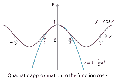
One graph. a. y = cos x, local minimums in quadrants 2 and 3, x intercepts at (-3π over 2, 0), (-π over 2, 0), (π over 2, 0), and (3π over 2, 0), y intercepts at (0,1).
b. y =1- one half x squared, concave parabola, turning point at (0,1), x intercepts at (-π over 2, 0) and (π over 2, 0).
Detailed description of diagram

If we continue on, we can find a cubic approximation to \(\cos x\) which agrees up to the third derivative at \(x=0\), a quartic which agrees up to the fourth derivative, and so on. In this way we get a sequence of polynomials which approximate \(\cos x\) increasingly better.

\[ \begin{array}{rclcl} \cos x & \sim & 1 & & \text{'constant' approximation} \\[2.5ex] &\sim & 1 - \dfrac{x^2}{2!} & & \text{quadratic approximation} \\[2.5ex] & \sim & 1 - \dfrac{x^2}{2!} + \dfrac{x^4}{4!} & & \text{quartic approximation} \\[2.5ex] & \sim & 1 - \dfrac{x^2}{2!} + \dfrac{x^4}{4!} - \dfrac{x^6}{6!} & & \text{degree-6 approximation} \end{array} \]

Continuing these terms on to infinity results in an infinite series approximating \(\cos x\). In fact this infinite series equals \(\cos x\):

\[ \cos x = 1 - \frac{x^2}{2!} + \frac{x^4}{4!} - \frac{x^6}{6!} + \frac{x^8}{8!} - \dots = \sum_{k=0}^\infty (-1)^k \frac{x^{2k}}{(2k)!}. \]

A series like this is known as a power series. Many functions can be well approximated by power series. Some are approximated completely and 'eventually exactly' like this one. For others, the power series only gives a good approximation in an interval of convergence. This topic is studied extensively in university science and engineering courses.

Next page - Links forward - Sums and products of roots