Content
Sketching polynomial functions
Although polynomial graphs come in many shapes and sizes, they can be sketched once we find a few of their features.
Example
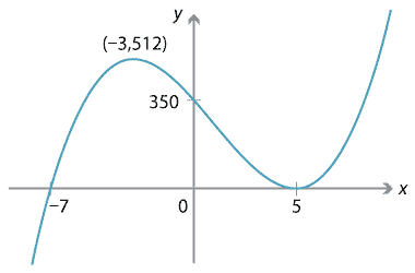
Sketch the graph of \(y=f(x)\) where \(f(x) = 2x^3 - 6x^2 - 90x +350\).
Solution
To find the \(x\)-intercepts, we solve \(f(x) = 2(x^3 - 3x^2 - 45x + 175) = 0\). Trying factors of 175 we find that \(x=5\) is a solution, so \((x-5)\) is a factor. We can then completely factorise \(f(x)\) as \(2(x-5)^2(x+7)\). So the \(x\)-intercepts are at \(x=5,-7\). To find the \(y\)-intercept, we compute \(f(0) = 350\).
To find the behaviour as \(x \to \pm \infty\), note that \(f(x)\) behaves like the leading term \(2x^3\). So \(f(x) \to +\infty\) as \(x \to +\infty\), and \(f(x) \to -\infty\) as \(x \to -\infty\).
To find the stationary points, we solve \(f'(x) = 0\). Differentiating gives
\[ f'(x) = 6x^2 - 12x - 90 = 6(x^2 - 2x - 15). \]Solving \(x^2 - 2x - 15 = 0\) gives \(x=-3,5\). Substituting these values into \(f\) gives \(f(-3) = 512\) and \(f(5) = 0\). So the stationary points are \((-3,512)\) and \((5,0)\).
From this information, we can sketch the graph of \(y=f(x)\).
Although it's unnecessary in the previous example, we could use a sign diagram to investigate stationary points. We choose values of \(x\) before and after each stationary point, and consider whether \(f'(x) = 6(x+3)(x-5)\) is positive or negative, as shown below.
| value of \(x\) | −3 | 5 | |||
|---|---|---|---|---|---|
| sign of \(f'(x)\) | + | 0 | − | 0 | + |
| slope of graph \(y=f(x)\) | \(\diagup\) | — | \(\diagdown\) | — | \(\diagup\) |
From the sign diagram we see directly that \(x=-3\) is a local maximum and \(x=5\) is a local minimum. However in the example this is deduced from other information.
In summary, the following information may be useful when sketching the graph of a polynomial \(y=f(x)\):
- \(x\)-intercepts, obtained by solving \(f(x)=0\)
- \(y\)-intercept, obtained by evaluating \(f(0)\)
- behaviour as \(x \to \pm \infty\), obtained by considering the leading term of \(f(x)\)
- stationary points, obtained by solving \(f'(x)=0\)
- sign diagram for \(f'(x)\), obtained by substituting values into \(f'(x)\).
It's not always necessary to calculate all of these; often, as in the previous example, a graph can be sketched with less information.
Repeated roots
When a polynomial has a factor \((x-a)\) to a power greater than 1, we say \(a\) is a repeated root. If \((x-a)^2\) is a factor of \(f(x)\), we say \(a\) is a double root or a root of multiplicity 2. In general, if \((x-a)^m\) is a factor of \(f(x)\), we say \(a\) is a root of multiplicity \(m\). A root of multiplicity 1 is often called a simple root.
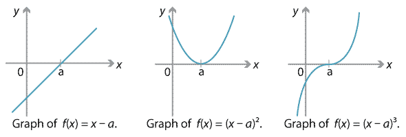
Consider the polynomial \(f(x) = (x-a)^m\), where \(a\) is a real number and \(m\) is a positive integer. Obviously \(f(x)\) has a root at \(x=a\) of multiplicity \(m\). The following three graphs show \(y=f(x)\) when \(m=1,2,3\).
Detailed description of diagrams
An important fact to note is that the sign of \(f(x)\) changes at \(x=a\) when \(m\) is odd, and does not change when \(m\) is even. (To see this, note that if \(x>a\), then \(x-a\) is positive and \((x-a)^m\) is also positive. If \(x<a\), then \(x-a\) is negative; if \(m\) is even, then \((x-a)^m\) is positive, while if \(m\) is odd, then \((x-a)^m\) is negative.)
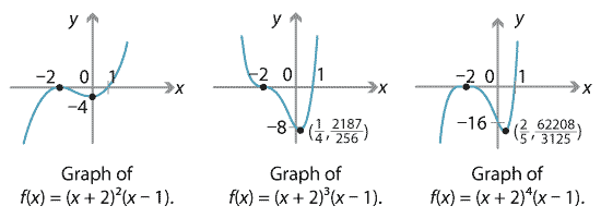
This fact becomes relevant when we consider more general polynomials with repeated roots. Consider the polynomials \(f(x) = (x+2)^m (x-1)\), where \(m\) is a positive integer. Then \(f(x)\) has a root at \(x=-2\) of multiplicity \(m\). The graphs for \(m=2,3,4\) are shown below.
Detailed description of diagrams
First consider the polynomial \(f(x) = (x+2)^2 (x-1)\), which has a double root at \(x=-2\). Then \(f(-2) = 0\). Since the power 2 is even, the factor \((x+2)^2\) does not change sign at \(x=-2\); if \(x\) is slightly more or less than \(-2\), then \((x+2)^2\) is positive. For \(x\) close to \(-2\), the factor \(x-1\) is negative, and so \(f(x)\) is negative for \(x\) slightly more or less than \(-2\). That is, \(f(x)\) does not change sign at \(x=-2\).
Next, consider \(f(x) = (x+2)^3 (x-1)\), which has a triple root at \(x=-2\). As 3 is odd, the factor \((x+2)^3\) does change sign at \(x=-2\). For \(x\) near \(-2\), the factor \(x-1\) is negative. So \(f(x)\) changes sign at \(x=-2\).
The above argument relies only on whether the multiplicity of the root \(x=-2\) is even or odd. Using a similar argument, one can prove the following theorem.
Screencast of interactive 5 ![]() ,
Interactive 5
,
Interactive 5 ![]()
Theorem
Let \(f(x)\) be a polynomial with a root \(a\) of multiplicity \(m\). Then \(f(x)\) changes sign at \(x=a\) if and only if \(m\) is odd.
If a polynomial \(f(x)\) has a root at \(x=a\) of even multiplicity \(m\), then \(f(x)\) does not change sign at \(x=a\), and yet \(f(a)=0\). Hence there must be a turning point and we obtain the next theorem.
Theorem
Let \(f(x)\) be a polynomial with a root \(a\) of even multiplicity. Then the graph of \(y=f(x)\) has a turning point at \(x=a\).
Additionally, we note from the above graphs that a root of multiplicity 2 or more always appears to be a stationary point. We can also prove this as a theorem.
Theorem
Let \(f(x)\) be a polynomial with a root \(a\) of multiplicity 2 or more. Then the graph of \({y=f(x)}\) has a stationary point at \(x=a\).
Proof
- Since \(a\) has multiplicity at least 2, we know that \((x-a)^2\) is a factor of \(f(x)\). (Maybe higher powers of \((x-a)\) divide into \(f(x)\), but \((x-a)^2\) certainly does.)
- We can then write \(f(x) = (x-a)^2 g(x)\) for some polynomial \(g(x)\). Differentiate \(f(x)\) using the chain and product rules to obtain
- Thus \(f'(a) = 0\) and so \(x=a\) is a stationary point. \(\Box\)
Transformation methods
We've seen from the module Functions II that, if we take the graph of \(y=f(x)\) and dilate or translate it in the \(x\) and \(y\) directions, or reflect in the axes, then the result is a graph of \(y=af(b(x-c))+d\), for some real numbers \(a,b,c,d\).We can sometimes use this idea in reverse, as in the following example. It's easier than using the standard method.
Example
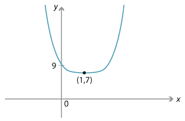
Sketch the graph of \(y=2 (x-1)^4 + 7\).
Solution
We see that the graph is obtained from \(y=x^4\) by successively:
- dilating by a factor of 2 from the \(x\)-axis in the \(y\)-direction
- translating 1 to the right
- translating 7 upwards.
Since we know the graph of \(y=x^4\), the graph is easily obtained.
Next page - Content - Polynomials from graphs
| This publication is funded by the Australian Government Department of Education, Employment and Workplace Relations |
Contributors Term of use |