Content
Behaviour of polynomials at infinity
Understanding the behaviour of a polynomial function \(f(x)\) when \(x\) is large (that is, as \(x \to \pm \infty\)) helps us to sketch the graph of \(y=f(x)\).
We've seen from examples that, for polynomial functions up to degree 4, the graph of a polynomial \(f(x) = a_n x^n + a_{n-1} x^{n-1} + \dots + a_0\) behaves asymptotically like its leading term \(a_n x^n\).
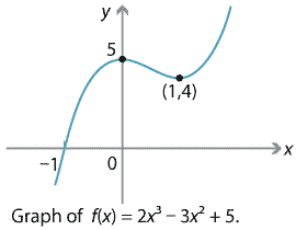
Let's consider how this behaviour arises. Take a cubic polynomial that we saw earlier, \(f(x) = 2x^3 - 3x^2 + 5\).
Detailed description of diagram
When \(x\) is large (positive or negative), \(x^2\) is much larger again, and \(x^3\) dwarfs them both. So the \(x^3\) term will 'dominate' the others. One way to see this algebraically is to write
\[ f(x) = 2x^3 - 3x^2 + 5 = 2x^3 \Big( 1 - \frac{3}{2x} + \frac{5}{2x^3} \Big). \]When \(x\) is large, both \(\dfrac{3}{2x}\) and \(\dfrac{5}{2x^3}\) become very small, and so effectively the dominant term is \(2x^3\). This explains why, as seen on the graph,
\[ f(x) \to + \infty \ \text{as} \ x \to +\infty, \qquad \text{and} \qquad f(x) \to - \infty \ \text{as} \ x \to -\infty. \]A similar argument applies to any polynomial \(f(x) = a_n x^n + a_{n-1} x^{n-1} + \dots + a_0\): for large \(x\), the \(a_n x^n\) term dominates the others.
Looking at the asymptotic behaviour, we can say that the graph \(y=x^n\) is roughly U-shaped when \(n\) is even, in the sense that \(x^n \to +\infty\) as \(x \to \pm \infty\). The actual graph may have many turning points, but if we imagine 'zooming out' and looking only at the large-scale picture when \(x\) is large, the graph is U-shaped. In a similar way, the graph of \(y=x^n\) is roughly /-shaped when \(n\) is odd. The behaviour of a polynomial graph \(y=f(x)\) when \(x\) is large will depend on whether the degree of \(f(x)\) is even or odd, and on the sign of the leading coefficient \(a_n\). We can summarise the outcomes, along with rough shapes of graphs when \(x\) is large, in a table.
| If \(n\) is | and \(a_n\) is | then as \(x \to +\infty\) | and as \(x \to -\infty\) | so shape is roughly |
|---|---|---|---|---|
| even | positive | \(f(x) \to +\infty\) | \(f(x) \to +\infty\) | |
| even | negative | \(f(x) \to -\infty\) | \(f(x) \to -\infty\) | |
| odd | positive | \(f(x) \to +\infty\) | \(f(x) \to -\infty\) | |
| odd | negative | \(f(x) \to -\infty\) | \(f(x) \to +\infty\) |
This confirms our Conjecture 5.
Example
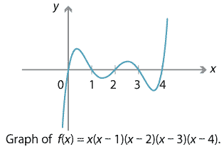
Sketch the graph of \(y= x(x-1)(x-2)(x-3)(x-4)\), marking all intercepts (but not turning points).
Solution
It's clear that the polynomial \(f(x) = x(x-1)(x-2)(x-3)(x-4)\) has roots at \(x=0,1,2,3,4\), and so these are the \(x\)-intercepts. The \(y\)-intercept is 0. Also, \(f(x)\) is a quintic polynomial with leading term \(x^5\). (This can be seen without fully expanding out the brackets.) Hence \(f(x)\) behaves like \(x^5\), for large~\(x\): as \(x \to + \infty\), \(f(x) \to +\infty\), and as \(x \to - \infty\), \(f(x) \to - \infty\). This is enough information to sketch the graph.
Finally, we can use the asymptotic behaviour of a polynomial \(f(x)\) to obtain information about its \(x\)-intercepts. When we have an odd-degree polynomial, the graph of \(y=f(x)\) must go from \(-\infty\) to \(+\infty\), or vice versa. Therefore the graph of \(y=f(x)\) must cross the \(x\)-axis, giving at least one \(x\)-intercept. This proves that the graph of a polynomial of odd degree has at least one \(x\)-intercept, confirming Conjecture 2.
Next page - Content - Stationary points
| This publication is funded by the Australian Government Department of Education, Employment and Workplace Relations |
Contributors Term of use |