Content

Polynomial function gallery

We can draw the graph of a polynomial function \(f(x)\) by plotting all points \((x,y)\) in the Cartesian plane with \(y\)-value given by \(f(x)\). In other words, we draw the graph of the equation \(y=f(x)\).

We will examine some graphs of polynomial functions. We'll start from simpler, low-degree polynomials, making some observations as we go.

We are very familiar with graphing polynomials of degree 0 or 1, i.e., constant or linear functions.

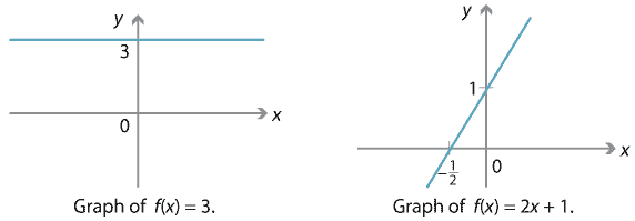
Detailed description of diagrams

Quadratics

We should also be comfortable with graphing polynomials of degree 2, i.e., quadratic functions. We know that we can always complete the square, so we can rewrite a quadratic function \(f(x) = ax^2 + bx + c\) as \(a(x-h)^2 + k\) for some constants \(h\) and \(k\). (Can you find a formula for \(h\) and \(k\) in terms of \(a,b,c\)?) As we know from the module Functions II, the graph of \(y=a(x-h)^2+k\) can be obtained from the standard parabola \(y=x^2\) by reflections, dilations and translations. In other words, any quadratic graph is a standard parabola, suitably reflected, dilated and translated.

In particular, the turning point of \(y=a(x-h)^2+k\) is at \((h,k)\).

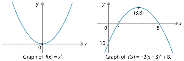
Detailed description of diagrams

The sign of \(a\) (whether positive or negative) determines the general shape of the graph. When \(a\) is positive, then as \(x \to \pm \infty\), we see that \(y \to \infty\), so the graph is curved like a smile ('happy'). If you imagine the graph as a road, and driving along it in the positive \(x\)-direction, you would always be turning left. (In the language of calculus, the derivative is increasing.) We say the graph is convex (or 'concave up').

On the other hand, when \(a\) is negative, then as \(x \to \pm \infty\), we have \(y \to -\infty\), so the graph is curved like a frown ('sad'). Driving along it in the positive \(x\)-direction, you would always be turning right, and the graph is concave (or 'concave down').

Cubics

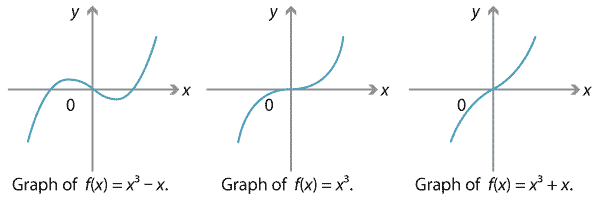
As we move from quadratic to cubic polynomials, things become more complicated. Unlike the situation with quadratics, not every cubic graph is obtained from the standard cubic graph \(y=x^3\) by reflections, dilations and translations. Indeed, if we consider three very simple cubic polynomials \(x^3 - x\), \(x^3\) and \(x^3 + x\), we get three distinct shapes.

Detailed description of diagrams

Note in particular the graph of \(y=x^3 + x\), which has no turning points and no stationary points of inflexion. This example shows that it's possible for a cubic graph to have no stationary points at all.

The graph of a cubic polynomial may have one, two or three \(x\)-intercepts. The examples above have one and three intercepts; below is an example with two of them.

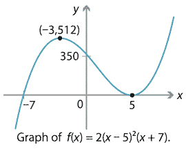
Detailed description of diagram

Note. On our graphs we mark turning points, stationary points of inflexion and intercepts where appropriate. We will have more to say about finding these points later on.

The behaviour of the above cubic graphs \(y=f(x)\) is not so different from that of \(y=x^3\), at least when \(x\) is large. If \(x\) is a large positive number, then \(f(x)\) is also a large positive number; if \(x\) is a large negative number, then \(f(x)\) is also a large negative number. Asymptotically, \(f(x)\) behaves similarly to \(x^3\).

However, in all the examples seen so far, the leading coefficient (i.e., the coefficient of \(x^3\)) has been positive. In the case that the leading coefficient is negative, the behaviour for large \(x\) is reversed. If \(x\) is a large positive number, then \(f(x)\) is a large negative number; if \(x\) is a large negative number, then \(f(x)\) is a large positive number. Below we graph the cubic polynomials \(-x^3 + x\), \(-x^3\) and \(-x^3 - x\), which all have a negative leading coefficient. Asymptotically, these cubic polynomials behave similarly to \(-x^3\).

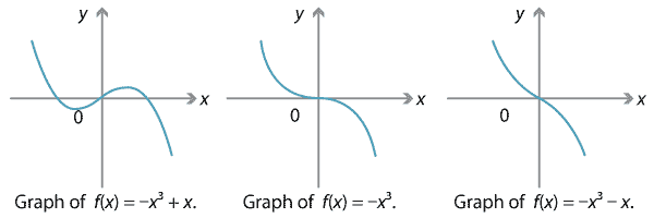
Detailed description of diagrams

It appears, then, that the leading term of a cubic polynomial determines its behaviour for large \(x\). In particular, a cubic graph goes to \(-\infty\) in one direction and \(+\infty\) in the other. So it must cross the \(x\)-axis at least once.

Furthermore, all the examples of cubic graphs have precisely zero or two turning points, an even number. (One way to see why: Think about moving along a cubic graph in the positive \(x\)-direction. Either you go up all the way, or you go down all the way, or you go up-down-up, or down-up-down. That's zero or two turns. Indeed, if you start going upwards, and you end going upwards, then you must have turned an even number of times.)

Screencast of exercise 3

In fact, when looking at the graph of a cubic polynomial \(f(x) = ax^3 + bx^2 + cx + d\), the number \(b^2 - 3ac\) tells us about the shape of the graph. Depending on whether this number is negative, zero or positive, the graph has zero, one or two stationary points. (We'll see why a little later on.)

Detailed description of diagrams

Notice that all the cubic graphs we have seen are quite symmetric. There is always a point on the graph about which the graph is symmetric under \(180^\circ\) rotation. This is true in general.

Screencast of interactive 1 ,  Interactive 1
Screencast of interactive 2 ,  Interactive 2

Quartics

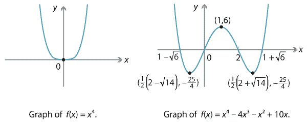
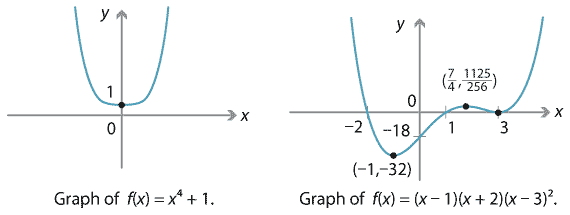
We turn next to quartic graphs, where an even wider variety of shapes is possible. First, consider the graph of the standard quartic \(f(x)=x^4\), which is something like a steeper and flatter version of a parabola, and the graph of \(f(x) = x^4 - 4x^3 - x^2 + 10x\), which has four \(x\)-intercepts.

Detailed description of diagrams

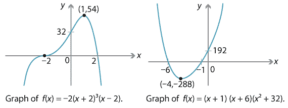
Note that both the graphs above are rather symmetric: they have vertical axes of symmetry at \(x=0\) and \(x=1\), respectively. (Compare the \(180^\circ\) rotational symmetry of cubic graphs.) However, not all quartic graphs are so symmetric. For instance, consider the following graphs of \(f(x) = -2(x+2)^3(x-2)\) and \(f(x)=(x+1)(x+6)(x^2 + 32)\).

Detailed description of diagrams

Both these graphs have two \(x\)-intercepts and only one turning point. The first has a stationary point of inflexion; the second does not. We can also obtain asymmetric W-shaped graphs, such as the following.

Detailed description of diagrams

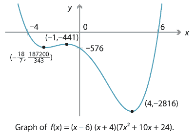
So far, we have seen quartic graphs with one, two or four \(x\)-intercepts. It's also possible to have zero or three \(x\)-intercepts, as shown below. We'll see that it's impossible to obtain five or more \(x\)-intercepts.

Detailed description of diagrams

All these quartics, for large \(x\), behave roughly like \(y=x^4\) or \(y=-x^4\) depending on the leading coefficient. When the leading coefficient is positive, then \(f(x) \to \infty\) as \(x\) becomes large (positive or negative). When the leading coefficient is negative, then \(f(x) \to -\infty\) as \(x\) becomes large. Again the leading term determines the asymptotic behaviour.

Screencast of interactive 4 ,  Interactive 4

Higher degree

As we consider quintics and higher, we will see more turning points, more \(x\)-intercepts and more points of inflexion. Let us summarise some of the observations we have made.

Graphs of polynomials

Type of polynomial	Number of \(x\)-intercepts	Number of turning points
linear	1	0
quadratic	from 0 to 2	1
cubic	from 1 to 3	0 or 2
quartic	from 0 to 4	1 or 3

We might make several conjectures based on these observations. We'll see why these are all true as we proceed. You can formulate more conjectures as well.

Conjectures

1. The graph of a polynomial of degree \(n\) has at most \(n\) \(x\)-intercepts.
2. The graph of a polynomial of odd degree has at least one \(x\)-intercept.
3. The graph of a polynomial of degree \(n\) has at most \(n-1\) turning points.
4. The graph of a polynomial of even degree has at least one turning point.
5. The graph of a polynomial \(f(x) = a_n x^n + a_{n-1} x^{n-1} + \dots + a_0\) behaves asymptotically like its leading term \(a_n x^n\). That is, when \(x\) is large (approaching \(+\infty\) or \(-\infty\)), \(f(x)\) has the same behaviour (approaching \(+\infty\) or \(-\infty\)) as \(a_n x^n\).

Next page - Content - Solving polynomial equations