Answers to exercises

Exercise 1

Let $T$ be the waiting time (in days) until the first call. Then $T \stackrel{\mathrm{d}}{=} \exp(1.8)$ , and therefore $F_T(t) = 1 - \exp(-1.8t)$ , for $t > 0$ . We need to be careful about the units of time used here.

$15$ minutes equals $\dfrac{15}{24 \times 60}$ days, or 0.01042 days. Hence, the chance of a call in the first 15 minutes equals $F_T(0.01042) = 1 - \exp(-1.8 \times 0.01042) = 0.0186$ .
Due to the lack of memory property, the probability is the same as that in part a, namely $0.0186$ .
$10$ hours equals $\dfrac{10}{24}$ days, or 0.41667 days. So the probability of no calls during a shift is $\Pr(T > 0.41667) = \exp(-1.8 \times 0.41667) = 0.4724$ .
Assuming independence between days, the probability of no calls in four successive days equals $0.4724^4 = 0.0498$ .
Solving for the time $y$ in days: $\begin{alignat*}{2} && \Pr(T \leq y) &= 0.1 \\\\ &\implies\quad& F_T(y) &= 0.1 \\\\ &\implies& 1 - \exp(-1.8y) &= 0.1 \\\\ &\implies& -1.8y &= \ln(0.9) \\\\ &\implies& y &= 0.0585 \text{ days}. \end{alignat*}$ Hence, $x$ is 1.4 hours, which is 1 hour 24 minutes.

Exercise 2

$f_X(\mu) = \dfrac{1}{\sigma \sqrt{2 \pi}} \approx \dfrac{0.40}{\sigma}$ .
We have $f_X(x) = f_X(\mu)\,\exp(k(x))$ , where $k(x) \leq 0$ for all values of $x$ . So $\exp(k(x)) \leq 1$ , and the result follows.
To find points of inflexion, we need the second derivative of $f_X(x)$ . Using the chain rule, we have $\begin{align*} f_X'(x) &= \dfrac{d}{dx}\Bigl[\dfrac{1}{\sigma \sqrt{2\pi}}\,\exp\bigl(\dfrac{-(x-\mu)^2}{2\sigma^2}\Bigr)\Bigr] \\\\ &= \dfrac{1}{\sigma \sqrt{2\pi}}\Bigl(\dfrac{-(x-\mu)}{\sigma^2}\Bigr)\;\exp\Bigl(\dfrac{-(x-\mu)^2}{2\sigma^2}\Bigr). \end{align*}$ Now, using the product rule, we have $f_X''(x) = \dfrac{1}{\sigma \sqrt{2\pi}}\Bigl[\dfrac{(x - \mu)^2}{\sigma^4}-\dfrac{1}{\sigma^2}\Bigr]\;\exp\Bigl(\dfrac{-(x-\mu)^2}{2\sigma^2}\Bigr).$ At a point of inflexion, $f_X''(x) = 0$ . This gives $\begin{alignat*}{2} && f_X''(x) &= 0 \\\\ &\implies\quad& \dfrac{(x-\mu)^2}{\sigma^4} - \dfrac{1}{\sigma^2} &= 0 \\\\ &\implies& (x - \mu)^2 &= \sigma^2 \\\\ &\implies& x &= \mu \pm \sigma. \end{alignat*}$ Hence, the points of inflexion are at $x = \mu - \sigma$ and $x = \mu + \sigma$ ; these are the points either side of $\mu$ at which the curve changes from convex to concave.

$f_X(\mu + k\sigma) = \dfrac{1}{\sigma \sqrt{2\pi}} \exp(-\dfrac{1}{2}k^2)$ .

$k$	1	1	2	3	4	5
$\exp(-\dfrac{1}{2}k^2)$	1	0.607	0.135	0.011	0.0003	0.000004

Note that $f_X(\mu - k\sigma) = f_X(\mu + k\sigma)$ , by symmetry.

There are a couple of useful interpretations:

Firstly, when sketching a Normal pdf, the height of the curve at $\mu \pm \sigma$ is 61% of the height of the central peak, and so on.
Second, recall that the height of a pdf reflects probabilities, so that if $f_X(b) = 2 f_X(a)$ , then the chance of an observation near $b$ is approximately twice as likely as an observation near $a$ . This means, for example, that observations near $\mu$ are approximately $250\ 000$ times more likely that observations near $\mu + 5 \sigma$ , since $\dfrac{1}{0.000004} = 250\ 0000$ .

Exercise 3

Let $D$ be the difference between the forecast maximum temperature and the actual maximum temperature (in degrees Celsius). Then $D \stackrel{\mathrm{d}}{=} \mathrm{N}(0,1.2^2)$ .

$\Pr(-1.0 < D < 1.0) = 0.595$ .
$\Pr(D < -0.5) = 0.338$ and $\Pr(-0.5 < D < 0.5) = 0.323$ , so it is very slightly more probable that there is an underestimate of 0.5 degrees or more.
We want to find the 0.01 quantile of the distribution; that is, we want $c_{0.01}$ satisfying $F_D(c_{0.01}) = 0.01$ . We find that $c_{0.01} = -2.79$ degrees. So 1% of forecast maximums are 2.79 degrees or more lower than the actual maximum. By symmetry, 1% of forecast maximums are 2.79 degrees or more higher than the actual maximum.

Exercise 4

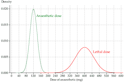
The pdfs of the random variables $A$ and $L$ are shown on the same axes in figure 6. The green distribution, on the left, is for the dose of anaesthetic required to render the animal unconscious. The average dose is 120 mg, and most values are in the range from about 60 mg to 180 mg. The red distribution, on the right, is for the lethal dose. The mean is 400 mg — much higher than the mean of the green distribution. There is little overlap of the two distributions. (Which is how we want things to be!) In fact, you might think that they do not overlap at all, based on a visual assessment of figure 6.

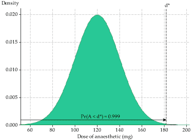
Figure 6: The pdfs of anaesthetic and lethal doses.
This question is about the anaesthetic dose administered, so we need to consider the distribution that renders animals suitably unconscious (the green distribution in figure 6). We need to find the value $d^*$ that corresponds to 99.9% of the animals being rendered suitably unconscious; this means a cumulative probability of 0.999. This is shown in figure 7.

Figure 7: The pdf of anaesthetic dose, showing $d^*$ .

We want to find $d^*$ such that $\Pr(A \leq d^*) = 0.999$ ; this is the 0.999 quantile of the distribution. This can be achieved in Excel using the function $\sf \text{NORM.INV}$ . If you enter $\sf \text{=NORM.INV(0.999, 120, 20)}$ in a cell, you should find that the dose required to render 99.9% of animals unconscious is $d^* = 181.80$ mg.
We now consider the distribution of the lethal dose, and what happens if a dose of 181.80 mg is administered. If a dose of 181.80 mg is used, there will be a small proportion of animals for whom this dose is lethal: those for whom the lethal dose is less than or equal to 181.80 mg. We are considering the pdf of $L$ (the red distribution in figure 6), and need to find the area under the curve corresponding to a dose of 181.80 or less. This is shown on the left in the following figure.

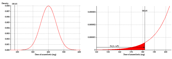
Figure 8: The pdf of lethal dose, showing $d^*$ .

The tail area is extremely small and hard to see, so the graph on the right is zoomed in to show the detail of the pdf of $L$ near $d^*$ .

To find the left-tail area in this distribution, we can use the cdf function in Excel; we enter $\sf \text{=NORM.DIST(181.80, 400, 50, 1)}$ in a cell. The value returned, and hence the proportion dying, is 0.0000064, or 0.00064%. This corresponds to 6 in a million, which is very small, as we suspect from the diagrams: a good result.