Content

Mean and variance of a continuous random variable

Mean of a continuous random variable

When introducing the topic of random variables, we noted that the two types — discrete and continuous — require different approaches.

In the module Discrete probability distributions , the definition of the mean for a discrete random variable is given as follows: The mean $\mu_X$ of a discrete random variable $X$ with probability function $p_X(x)$ is

\[ \mu_X = \mathrm{E}(X) = \sum x\,p_X(x), \]

where the sum is taken over all values $x$ for which $p_X(x) > 0$.

The equivalent quantity for a continuous random variable, not surprisingly, involves an integral rather than a sum. The mean $\mu_X$ of a continuous random variable $X$ with probability density function $f_X(x)$ is

\[ \mu_X = \mathrm{E}(X) = \int_{-\infty}^{\infty} x\,f_X(x)\;dx. \]

By analogy with the discrete case, we may, and often do, restrict the integral to points where $f_X(x) > 0$.

Several of the points made when the mean was introduced for discrete random variables apply to the case of continuous random variables, with appropriate modification.

Recall that mean is a measure of 'central location' of a random variable. It is the weighted average of the values that $X$ can take, with weights provided by the probability density function. The mean is also sometimes called the 'expected value' or 'expectation' of $X$ and denoted by $\mathrm{E}(X)$. In visual terms, looking at a pdf, to locate the mean you need to work out where the pivot should be placed to make the pdf balance on the $x$-axis, imagining that the pdf is a thin plate of uniform material, with height $f_X(x)$ at $x$.

An important consequence of this is that the mean of any symmetric random variable (continuous or discrete) is always on the axis of symmetry of the distribution; for a continuous random variable, this means the axis of symmetry of the pdf.

Exercise 3

Two triangular pdfs are shown in figure 9.

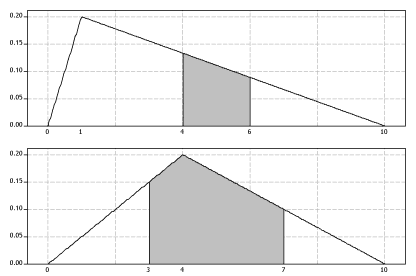
The probability density functions of two continuous random variables.

Figure 9: The probability density functions of two continuous random variables.

Each of the pdfs is equal to zero for $x<0$ and $x>10$, and the $x$-values of the apex and the boundaries of the shaded region are labelled on the $x$-axis in figure 9.

For each of these pdfs separately:

Write down a formula (involving cases) for the pdf.
Guess the value of the mean. Then calculate it to assess the accuracy of your guess.
Guess the probability that the corresponding random variable lies between the limits of the shaded region. Then calculate the probability to check your guess.

The module Discrete probability distributions gives formulas for the mean and variance of a linear transformation of a discrete random variable. In this module, we will prove that the same formulas apply for continuous random variables.

Theorem

Let $X$ be a continuous random variable with mean $\mu_X$. Then

\[ \mathrm{E}(aX + b) = a\,\mathrm{E}(X) + b = a\mu_X + b, \]

for any real numbers $a,b$.

Proof

For a continuous random variable $X$, the mean of a function of $X$, say $g(X)$, is given by

\[ \mathrm{E}[g(X)] = \int_{-\infty}^{\infty} g(x)\,f_X(x)\;dx. \]

So, for $g(X) = aX + b$, we find that

\begin{align*} \mathrm{E}(aX+b) &= \int_{-\infty}^{\infty} (ax+b)\,f_X(x)\;dx \\\\ &= \int_{-\infty}^{\infty} ax\,f_X(x)\;dx + \int_{-\infty}^{\infty} b\,f_X(x)\;dx \\\\ &= a \int_{-\infty}^{\infty} x\,f_X(x)\;dx + b \int_{-\infty}^{\infty} f_X(x)\;dx \\\\ &= a\mu_X + b. \end{align*}

$\Box$

Variance of a continuous random variable

Recall that the variance of a random variable $X$ is defined as follows:

\[ \mathrm{var}(X) = \sigma_X^2 = \mathrm{E}[(X - \mu)^2], \qquad\text{where } \mu = \mathrm{E}(X). \]

The variance of a continuous random variable $X$ is the weighted average of the squared deviations from the mean $\mu$, where the weights are given by the probability density function $f_X(x)$ of $X$. Hence, for a continuous random variable $X$ with mean $\mu_X$, the variance of $X$ is given by

\[ \mathrm{var}(X) = \sigma_X^2 = \mathrm{E}[(X - \mu_X)^2] = \int_{-\infty}^{\infty} (x-\mu_X)^2 f_X(x)\;dx. \]

Recall that the standard deviation $\sigma_X$ is the square root of the variance; the standard deviation (and not the variance) is in the same units as the random variable.

Exercise 4

Find the standard deviation of

the random variable $U \stackrel{\mathrm{d}}{=} \mathrm{U}(0,1)$; see figure 6
the random variable $V$ from exercise 2.

As observed in the module Discrete probability distributions , there is no simple, direct interpretation of the variance or the standard deviation. (The variance is equivalent to the 'moment of inertia' in physics.) However, there is a useful guide for the standard deviation that works most of the time in practice. This guide or 'rule of thumb' says that, for many distributions, the probability that an observation is within two standard deviations of the mean is approximately 0.95. That is,

\[ \Pr(\mu_X - 2\sigma_X \leq X \leq \mu_X + 2\sigma_X) \approx 0.95. \]

This result is correct (to two decimal places) for an important distribution that we meet in another module, the Normal distribution, but it is found to be a useful indication for many other distributions too, including ones that are not symmetric.

Due to Chebyshev's theorem, not covered in detail here, we know that the probability $\Pr(\mu_X - 2\sigma_X \leq X \leq \mu_X + 2\sigma_X)$ can be as small as 0.75 (but no smaller) and it can be as large as 1. So clearly, the rule does not apply in some situations. But these extreme distributions arise rather infrequently across a broad range of practical applications.

Exercise 5

For the random variable $V$ from exercises 2 and 4, find $\Pr(\mu_V - 2\sigma_V \leq V \leq \mu_V + 2\sigma_V)$.

We now consider the variance and the standard deviation of a linear transformation of a random variable.

Theorem

Let $X$ be a random variable with variance $\sigma_X^2$. Then

\[ \mathrm{var}(aX + b) = a^2\,\mathrm{var}(X) = a^2\,\sigma_X^2, \]

for any real numbers $a,b$.

Proof

Define $Y = aX+b$. Then $\mathrm{var}(Y) = \mathrm{E}[(Y - \mu_Y)^2]$. We know that $\mu_Y = a\mu_X + b$. Hence,

\begin{align*} \mathrm{var}(aX+b) &= \mathrm{E}\bigl[\bigl(aX+b - (a\mu_X + b)\bigr)^2\bigr] \\\\ &= \mathrm{E}\bigl[a^2(X - \mu_X)^2\bigr] \\\\ &= a^2\,\mathrm{E}[(X - \mu_X)^2] \\\\ &= a^2\,\mathrm{var}(X) \\\\ &= a^2\,\sigma_X^2. \end{align*}

$\Box$

It follows from this result that

\[ \mathrm{sd}(aX+b) = |a|\,\mathrm{sd}(X) = |a|\,\sigma_X. \]

Exercise 6

Suppose that $X$, the distance travelled by a taxi in a single trip in a major Australian city, has a mean of 15 kilometres and a standard deviation of 50 kilometres. Define $Y$ to be the charge for a single trip (or, to be pedantic, the component of the charge that depends on flagfall and distance travelled). If the flagfall is $3.20 and the rate per kilometre is $2.20, what are the mean and the standard deviation of $Y$?

Next page - Content - Relative frequencies and continuous distributions