Content

Probability density functions

The probability density function (pdf) \(f(x)\) of a continuous random variable \(X\) is defined as the derivative of the cdf \(F(x)\):

\[ f(x) = \dfrac{d}{dx}F(x). \]

It is sometimes useful to consider the cdf \(F(x)\) in terms of the pdf \(f(x)\):

\[ F(x) = \int_{-\infty}^{x} f(t)\;dt. \qquad\qquad(\ast) \]

The pdf \(f(x)\) has two important properties:

\(f(x) \geq 0\), for all \(x\)
\(\displaystyle\int_{-\infty}^{\infty} f(x)\;dx = 1\).

The first property follows from the fact that the cdf \(F(x)\) is non-decreasing and \(f(x)\) is its derivative. The second property follows from equation (\(\ast\)) above, since \(F(x) \to 1\) as \(x \to \infty\), and so the total area under the graph of \(f(x)\) is equal to 1.

An infinite variety of shapes are possible for a pdf, since the only requirements are the two properties above. The pdf may have one or several peaks, or no peaks at all; it may have discontinuities, be made up of combinations of functions, and so on. figure 5 shows a pdf with a single peak and some mild skewness. As is the case for a typical pdf, the value of the function approaches zero as \(x \to \infty\) and \(x \to -\infty\).

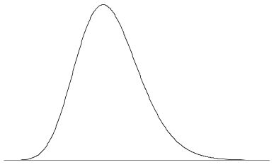
A continuous PDF with some mild skewness.
Figure 5: A pdf may look something like this.

We now explore how probabilities concerning the continuous random variable \(X\) relate to its pdf. The important result here is that

\[ \Pr(a < X \leq b) = \int_a^b f(x)\;dx = \bigl[ F(x) \bigr]_a^b. \]

This result follows from the fact that both sides are equal to \(F(b) - F(a)\).

Notes.

For a continuous random variable, we must consider the probability that it lies in an interval. The importance of this result is that it tells us that, to find the probability, we need to find the area under the pdf on the given interval.
The total area under the pdf equals 1. So this result tells us that, to approximate the probability that the random variable lies in a given interval, we just have to guess the fraction of the area under the pdf between the ends of the interval.
This result provides another perspective on why pdfs cannot be negative, since if they were, a negative probability could be obtained, which is impossible.
The pdf is analogous to, but different from, the probability function (pf) for a discrete random variable. A pf gives a probability, so it cannot be greater than one. A pdf \(f(x)\), however, may give a value greater than one for some values of \(x\), since it is not the value of \(f(x)\) but the area under the curve that represents probability. On the other hand, the height of the curve reflects the relative probability. If \(f(b) = 2f(a)\), then an observation near \(b\) is approximately twice as likely as an observation near \(a\).

Exercise 1

Consider the function

\[ f(x) = \begin{cases} 6x(1-x) &\text{if } 0 \leq x \leq 1, \\\\ 0 &\text{otherwise.} \end{cases} \]

Check that \(f(x)\) has the two required properties for a pdf, and sketch its graph.
Suppose that the continuous random variable \(X\) has the pdf \(f(x)\). Obtain the following probabilities without calculation:
1. \(\Pr(X \leq -3)\)
2. \(\Pr(0 \leq X \leq 1)\)
3. \(\Pr(0.5 \leq X \leq 1)\).
By looking at the graph of the pdf, guess the value of \(\theta = \Pr(0.4 \leq X \leq 0.7)\). Then check the accuracy of your guess by calculating \(\theta\).
1. Find \(f(0.2)\) and \(f(0.4)\), and hence obtain \(\lambda = \dfrac{f(0.4)}{f(0.2)}\).
2. Find the probability that \(X\) is within 0.05 of 0.2. That is, find the probability \(p_{0.2} = \Pr(0.15 \leq X \leq 0.25)\).
3. Find the probability that \(X\) is within 0.05 of 0.4. That is, find the probability \(p_{0.4} = \Pr(0.35 \leq X \leq 0.45)\).
4. Confirm that the ratio of these two probabilities is approximately equal to \(\lambda\). That is, check that \(\dfrac{p_{0.4}}{p_{0.2}} \approx \dfrac{f(0.4)}{f(0.2)}\).

Example: Random numbers, continued

Consider the continuous random variable \(U\) from the first random-number example. Then \(U \stackrel{\mathrm{d}}{=} \mathrm{U}(0,1)\). The pdf of \(U\) is given by

\[ f_U(u) = \begin{cases} 1 &\text{if } 0 < u < 1, \\\\ 0 &\text{otherwise.} \end{cases} \]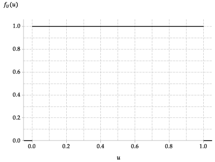

Figure 6: The probability density function of \(U \stackrel{\mathrm{d}}{=} \mathrm{U}(0,1)\).

Exercise 2

Consider the function \(f_V\) shown in figure 7; assume that \(f_V(v) = 0\) for \(v<0\) and \(v>1\).

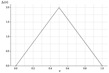
Figure 7: The probability density function of a random variable \(V\) with the triangular distribution.

Verify that \(f_V\) is a pdf.
Give a formula (involving cases) for the function \(f_V(v)\).
Suppose a continuous random variable \(V\) has this pdf. Find the cdf \(F_V(v)\) of \(V\).
Find \(\Pr(0.2 \leq V \leq 0.3)\).
Which is more likely: \(V \approx 0.3\) or \(V \approx 0.8\)? Explain.

The triangular pdf shown in figure 7 is the pdf of the average of two \(\mathrm{U}(0,1)\) random variables. That is, if \(U_1 \stackrel{\mathrm{d}}{=} \mathrm{U}(0,1)\) and \(U_2 \stackrel{\mathrm{d}}{=} \mathrm{U}(0,1)\) are independent, then \(V = \dfrac{1}{2}(U_1 + U_2)\) has the pdf in figure 7.

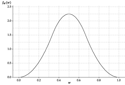
This raises the question: What does the average of three independent \(\mathrm{U}(0,1)\) random variables look like? The answer is shown in figure 8. If \(U_i \stackrel{\mathrm{d}}{=} \mathrm{U}(0,1)\), for \(i=1,2,3\), and the three random variables are independent, then \(W = \dfrac{1}{3}(U_1 + U_2 + U_3)\) has the following pdf.

Detailed description

Figure 8: The probability density function of \(W\), the average of three independent \(\mathrm{U}(0,1)\) random variables.

Next page - Content - Mean and variance of a continuous random variable