Content
Assigning probabilities
So far we have said little about how probabilities can be assigned numerical values in a random procedure. We know that probabilities must be in the interval \([0,1]\), but how do we know what the actual numerical value is for the probability of a particular event?
Symmetry and random mixing
Ideas for the assignment of probabilities have been progressively developed in earlier years of the curriculum. One important approach is based on symmetry. The outcome of rolling a fair die is one of the most common examples of this. Even small children will readily accept the notion that the probability of obtaining a three, when rolling a fair die, is \(\dfrac{1}{6}\). Where does this idea come from, and what assumptions are involved?
A classic 'fair die' is a close approximation to a uniform cube. (The word 'approximation' is used here because many dice have slightly rounded corners and edges.) A cube, by definition, has six equal faces, all of which are squares. So if we roll the die and observe the uppermost face when it has come to rest, there are six possible outcomes. The symmetry of the cube suggests there is no reason to think that any of the outcomes is more or less likely than any other. So we assign a probability of one sixth to each of the possible outcomes. Here \(\mathcal{E} = \{1,2,3,4,5,6\}\) and \(\Pr(i) = \dfrac{1}{6}\), for each \(i = 1,2,\dots,6\).
What assumptions have we made here? One important aspect of this process is the rolling of the die. Suppose my technique for 'rolling' the die is to pick it up and turn it over to the opposite face. This cannot produce all six outcomes. Furthermore, the two outcomes that are produced by this process occur in a non-random systematic sequence.
So we observe that, with randomising devices such as coins, dice and cards, there is an important assumption about random mixing involved. When playing games like Snakes and Ladders that use dice, we are familiar with players shaking the cup extra vigorously in the interests of a truly random outcome, and on the other hand, those trying to slide the die from the cup in order to produce a six!
Exercise 5
Consider each of the following procedures. How random do you think the mixing is likely to be?
- A normal coin flip that lands on your hand.
- A normal coin flip that lands on the floor.
- A die shaken vigorously inside a cup 'sealed' at the top by your palm, then rolled onto the table.
- An 'overhand' shuffle of cards; this is the shuffle that we usually first learn.
- A 'riffle' shuffle of cards: in this shuffle, two piles of cards are rapidly and randomly interwoven by gradual release from the two thumbs.
- The blast of air blown into the sphere containing the balls in Powerball.
- The random number generator that produces the next Tetris shape.
- The hat used for drawing raffles at the footy club.
For a guide to various card shuffles (including the overhand and riffle shuffles), www.pokerology.com/poker-articles/how-to-shuffle-cards ![]()
There are also more subtle aspects of symmetry to be considered. In the case of a conventional die, the shape may be cubical and hence symmetrical. But is that enough? We also need uniform density of the material of the cube, or at least an appropriately symmetric distribution of mass (some dice are hollow, for example). If a wooden die is constructed with a layer of lead hidden under one face, this would violate the assumption that we make in assigning equal probabilities to all six outcomes.
What about coin tossing and symmetry? We may assume that the coin itself is essentially a cylinder of negligible thickness made from uniform density metal with two perfectly flat sides. No actual coin is like this. The faces of coins have sculpted shapes on them that produce the images we see. These shapes are clearly not actually symmetric. How much does this matter?
Exercise 6
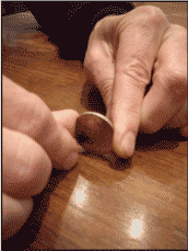
Starting position for
non-standard spin.
Use an ordinary 20 cent coin to carry out the following experiment. Find the flattest surface you can. Starting with the coin on its edge, spin the coin fast; usually this is most effectively done by delivering the spin from the index finger of one hand on one side of the coin against the thumb of the other hand on the other side, as shown in the photo.
The spin needs to be uninterrupted by other objects and stay on the flat surface throughout. There is a bit of skill required to get the coin to spin rapidly; practise until you can get it to spin for about ten seconds before coming to rest.
Once you are adept at this technique, on a given spin you can save time near the end of the spin: when it is clear what the result will be, you can stop the motion and record it. Do this 30 times. How many heads and tails do you get?
When we use symmetry to assign probabilities, it is important that the outcomes we consider are truly symmetric, and not just superficially so. It is definitely not enough to know merely the number of possible outcomes of a random process. Just because there are only \(k\) possible outcomes does not imply that each one of them has probability equal to \(\dfrac{1}{k}\); there needs to be a basis for assuming symmetry. Often a list of possible 'outcomes' is really a list of events, rather than elementary events. In that case, even if the elementary events are equiprobable, there is no need for the derived events to be so.
Exercise 7
A standard deck of cards is well shuffled and from it I am dealt a hand of four cards. In my hand I can have 0, 1, 2, 3 or 4 aces: five possibilities altogether. So the chance that my hand has four aces is equal to \(\dfrac{1}{5} = 0.2\).
What is wrong with this argument?
Relative frequencies
A second way to assign numerical values for probabilities of events is by using relative frequencies from data. In fact, this is probably the most common method. Strictly speaking, what we are doing is estimating probabilities rather than assigning the true numerical values.
For example, we may have data from 302 incidents in which school children left their bag at the bus stop briefly to run home and get something that they forgot. In 38 of these incidents, the bag was not there when they returned. So we might estimate the probability of losing a school bag as
\[ \dfrac{38}{302} \approx 0.126, \] or \(12.6\%\) on the percentage scale.Equally probable outcomes
There are many contexts in which it is desirable to ensure equal probabilities of outcomes. These include commercial games of chance, such as lotteries and games at casinos, and the allocation of treatments to patients in randomised controlled trials. Randomising devices are used to achieve this.
Example: Election ballots (California)
It is understood that there is a 'positional bias' in the voting behaviour of undecided voters in elections; that is, some of them tend to give their voting preference in the order that the candidates are listed on the ballot paper.
For this reason, in California, about three months before an election, the Secretary of State produces a random ordering of the letters of the alphabet. This is used to define the order in which the names of candidates are printed on the ballot papers. What's more, it is applied not just to the first letter of each candidate's name, but to the other letters in the names also.
Example: Powerball
The commercial lottery Powerball has operated in Australia since 1996. There are 45 balls that can appear as the Powerball. A probability model based on symmetry and random mixing implies that the chance of any particular ball appearing as the Powerball is \(\dfrac{1}{45} \approx 0.022\). (We are rounding to three decimal places here.) This is the idealised model that is intended on grounds of fairness for those who play the game, and we may believe that the model applies, to a very good approximation. There are laws governing lotteries that aim to ensure this.
At the time of writing, there have been 853 Powerball draws. The following table shows the relative frequencies of some of the 45 numbers from the 853 draws.
| Powerball | 1 | 2 | 3 | 4 | 5 | \(\dots\) | 43 | 44 | 45 |
|---|---|---|---|---|---|---|---|---|---|
| Relative frequency |
\(\dfrac{21}{853}\) | \(\dfrac{14}{853}\) | \(\dfrac{20}{853}\) | \(\dfrac{21}{853}\) | \(\dfrac{15}{853}\) | \(\dots\) | \(\dfrac{19}{853}\) | \(\dfrac{22}{853}\) | \(\dfrac{22}{853}\) |
| 0.025 | 0.016 | 0.023 | 0.025 | 0.018 | \(\dots\) | 0.022 | 0.026 | 0.026 |
We may check assumptions about randomness by looking at the relative frequencies. We may ask: Are they acceptably close to the probability implied by a fair draw, which is 0.022? Obviously, if we are to do this properly, we must look at the whole distribution, and not just the part shown here.
The previous example is related to testing in statistical inference, in which a model for a random process is proposed and we examine data to see whether it is consistent with the model. This is not part of the topic of probability directly, but it indicates one way in which probability models are used in practice.
Exercise 8
During the Vietnam War, the Prime Minister Robert Menzies introduced conscription to national army service for young men. However, not all eligible men were conscripted: there was a random process involved. Two birthday ballots a year were held to determine who would be called up. Marbles numbered from 1 to 366 were used, corresponding to each possible birthdate. The marbles were placed in a barrel and a predetermined number were drawn individually and randomly by hand. There were two ballots per year, the first for birthdates from 1 January to 30 June and the second for birthdates from 1 July to 31 December. In a given half year, if a birthdate was drawn, all men turning 20 on that date in that year were required by law to present themselves for national service. This occurred from 1965 until 1972, when Gough Whitlam's ALP government abolished the scheme.
Were men born on 29 February more likely to be conscripted, or less likely? Or were their chances the same as other men? What assumptions have you made?
- For a photo of the marbles, see https://vrroom.naa.gov.au/print/?ID=19537

- For the selected birthdates, see https://www.awm.gov.au/encyclopedia/viet_app/
A previous example described the method used to ensure electoral fairness in California. The next example concerns an issue of electoral fairness in Australia.
Example: Election ballots (Australian Senate, 1975)
The 1975 Senate election in Australia occurred in a heightened political climate. The Australian Labor Party (ALP) government, voted into power in 1972 and returned in 1974, was losing popularity. In November 1975, the government was dismissed by the Governor-General, Sir John Kerr, and an election was called which involved a 'double dissolution' of both houses of parliament. Between the dismissal on 11 November and the elections on 13 December, there were many protests, demonstrations and hot political debates. In the election for the Senate, the two main political parties were the ALP and the Liberal--National coalition; between them, they received 80% of the votes cast.
The following table gives some data from the draws for positions on the ballot papers in this Senate election. The table shows the positions of the Liberal--National coalition (L/N) and the ALP for each of the six states and two territories. Also shown in each case is the number of groups participating in the election. In WA and Tasmania, the Liberal Party and the National Party were separate; elsewhere they had a joint Senate team.
| State or territory | Position of | Number of groups | |
|---|---|---|---|
| L/N | ALP | ||
| NSW | 2 | 8 | 10 |
| Vic | 1 | 6 | 8 |
| Qld | 2 | 6 | 7 |
| SA | 1 | 3 | 9 |
| WA | 7,1 | 10 | 11 |
| Tas | 1,2 | 5 | 6 |
| ACT | 1 | 2 | 4 |
| NT | 1 | 3 | 3 |
The positions on each ballot paper were determined by drawing envelopes out of a box. Does the result of this appear to you to be appropriately random?
Among those who noted the strangeness of this distribution were two astute Melbourne statisticians, Alison Harcourt and Malcolm Clark. Their analysis of this result formed the basis of a submission to the Joint Select Committee on Electoral Reform in 1983, and this eventually led to a change in the Commonwealth Electoral Act. The process now involves much more thorough random mixing, using 'double randomisation' and a process similar to that used in Tattslotto draws.
Reference
R. M. Clark and A. G. Harcourt, 'Randomisation and the 1975 Senate ballot draw', The Australian Journal of Statistics 33 (1991), 261--278.
Next page - Content - Conditional probability
| This publication is funded by the Australian Government Department of Education, Employment and Workplace Relations |
Contributors Term of use |