Content

Estimates of area

Left-endpoint estimate

In the previous section, we estimated the area under the graph by splitting the interval $[0,5]$ into equal subintervals, and considering rectangles built on these subintervals. These rectangles had their top-left corner touching the curve $y=f(x)$. In other words, the height of the rectangle over a subinterval was the value of $f$ at the left endpoint of that subinterval. For this reason, this method is known as the left-endpoint estimate.

To obtain a general formula for this estimate, suppose we have a real-valued function $f(x)$ defined on an interval $[a,b]$. In order to estimate the area under the graph $y=f(x)$ between $x=a$ and $x=b$, we split $[a,b]$ into $n$ equal subintervals. Let these be

$$[x_0, x_1], \qquad [x_1, x_2], \qquad [x_2, x_3], \qquad \dots, \qquad [x_{n-1}, x_n].$$

So $x_0 = a$, $x_n = b$ and the real numbers $x_1, \dots, x_{n-1}$ are equally spaced between $a$ and $b$. As the numbers are equally spaced, the width of each interval is $\frac{1}{n} (b-a)$. That is,

$$x_j - x_{j-1} = \frac{b-a}{n}, \qquad \text{for all \(j=1, 2, \dots, n\)}.$$

We also write $\Delta x$ for this width, the 'change in $x$' between successive endpoints.

Above the interval $[x_0, x_1]$, we have a rectangle whose width is $\Delta x$ and whose height is $f(x_0)$. In general, above the interval $[x_{j-1},x_j]$, we have a rectangle of width $\Delta x$ and height $f(x_{j-1})$. The area of this rectangle is then $f(x_{j-1}) \; \Delta x$. The total area estimate is therefore

$$\big[ f(x_0) + f(x_1) + \dots + f(x_{n-1}) \big] \, \Delta x = \sum_{j=1}^n f(x_{j-1}) \; \Delta x.$$

Right-endpoint estimate

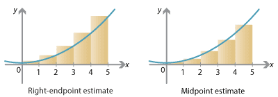
Instead of setting the height of each rectangle to the value of $f$ at the left endpoint of each subinterval, we can use the right endpoint and obtain the right-endpoint estimate.

We again have a rectangle above each interval $[x_{j-1},x_j]$ of width $\frac{1}{n} (b-a) = \Delta x$, but the height is now given at the right endpoint, i.e., the height is $f(x_j)$. So the total area estimate is

$$\big[ f(x_1) + f(x_2) + \dots + f(x_n) \big] \, \Delta x = \sum_{j=1}^n f(x_j) \; \Delta x.$$

Note that this formula only differs slightly from that for the left-endpoint estimate; the heights are obtained at $x$-values $x_1$ to $x_n$, rather than $x_0$ to $x_{n-1}$.

Detailed description of diagram

Screencast of interactive 2 ,  Interactive 2

Midpoint estimate

Screencast of interactive 3 ,  Interactive 3

A third way to estimate the area under a graph is to set the height of each rectangle equal to the value of $f$ at the midpoint of each subinterval, obtaining the midpoint estimate.

Specifically, above the interval $[x_0, x_1]$ there is again a rectangle of width $\Delta x$, but its height is the value of $f$ at the midpoint of the interval. The midpoint is $\frac{1}{2} (x_0 + x_1)$, so the height is $f \big( \frac{1}{2} (x_0+x_1) \big)$ and the area of the rectangle is $f \big( \frac{1}{2} (x_0+x_1) \big) \; \Delta x$. Similarly, above each interval $[x_{j-1},x_j]$, which has midpoint $\frac{1}{2} (x_{j-1}+x_j)$, there is a rectangle of width $\Delta x$ and height $f \big( \frac{1}{2} (x_{j-1} + x_j)\big)$, and hence of area $f \big( \frac{1}{2} (x_{j-1} + x_j) \big)\; \Delta x$. Therefore the total area estimate is

$$\Big[ f \Big( \frac{x_0+x_1}{2} \Big) + f \Big( \frac{x_1 + x_2}{2} \Big) + \dots + f \Big( \frac{x_{n-1} + x_n}{2} \Big) \Big] \, \Delta x = \sum_{j=1}^n f \Big( \frac{x_{j-1} + x_j}{2} \Big) \; \Delta x.$$

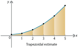
Trapezoidal estimate

We need not restrict ourselves to rectangles. Instead, we could plot the points on the graph $y=f(x)$ for each $x_j$, and join the dots. In this way, the function $f(x)$ is approximated by a piecewise linear function, that is, a sequence of straight line segments. The area under $y=f(x)$ is then approximated by trapezia. This estimate is known as the trapezoidal estimate.

Detailed description of diagram

Above the interval $[x_0, x_1]$ we have a trapezium of width $\frac{1}{n} (b-a) = \Delta x$. Its left side has height $f(x_0)$, and its right side has height $f(x_1)$. So the area of the trapezium is

$$\Big (\frac{f(x_0) + f(x_1)}{2} \Big) \; \Delta x.$$

Similarly, above the interval $[x_{j-1}, x_j]$, we have a trapezium of width $\Delta x$ with two sides of height $f(x_{j-1})$ and $f(x_j)$, hence the area of the trapezium is $\frac{1}{2} \big(f(x_{j-1}) + f(x_j) \big) \; \Delta x$. The total area estimate is

$$\Bigg[ \frac{f(x_0) + f(x_1)}{2} + \frac{f(x_1) + f(x_2)}{2} + \frac{f(x_2) + f(x_3)}{2} + \dotsb + \frac{f(x_{n-1}) + f(x_n)}{2} \Bigg] \, \Delta x,$$

which simplifies to

$$\Bigg[ \frac{1}{2} f(x_0) + f(x_1) + f(x_2) + \dotsb + f(x_{n-1}) + \frac{1}{2} f(x_n) \Bigg] \, \Delta x.$$

Screencast of interactive 1 ,  Interactive 1

Screencast of exercise 4

Limits of estimates

In some simple cases, it is possible to calculate an area estimate with $n$ rectangles (or trapezia) and explicitly take the limit as $n \to \infty$ to obtain the exact area. In the rest of this module, and in practice, we use other techniques to calculate areas, but it is worth seeing that sometimes a direct approach is possible.

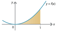
For example, consider the function $f(x) = x^2$ and the area under the graph $y=f(x)$ between $x=0$ and $x=1$. We'll compute the right-endpoint estimate with $n$ rectangles, and then take the limit as $n \to \infty$.

Dividing the interval $[0,1]$ into $n$ subintervals $[x_0, x_1]$, $\dots$, $[x_{n-1}, x_n]$, we have

$$\Delta x = \frac{1}{n} \qquad \text{and} \qquad x_j = \frac{j}{n}.$$

So the right-endpoint estimate is

$$\begin{align*} \sum_{j=1}^n f(x_j) \; \Delta x &= \sum_{j=1}^n f \Big( \frac{j}{n} \Big) \; \frac{1}{n}\\ &= \sum_{j=1}^n \Big( \frac{j}{n} \Big)^2 \; \frac{1}{n} = \frac{1}{n^3} \sum_{j=1}^n j^2. \end{align*}$$

As it turns out, there is a formula for the sum of the first $n$ squares:

$$\sum_{j=1}^n j^2 = 1^2 + 2^2 + \dots + n^2 = \frac{n(n+1)(2n+1)}{6}.$$

The right-endpoint estimate with $n$ rectangles then becomes

$$\begin{align*} \frac{n(n+1)(2n+1)}{6 n^3} &= \frac{2n^3 + 3n^2 + n}{6n^3}\\ &= \frac {1}{6} \, \Big(2 + \frac{3}{n} + \frac{1}{n^2}\Big). \end{align*}$$

Taking the limit as $n \to \infty$, since $\frac{3}{n} \to 0$ and $\frac{1}{n^2} \to 0$, the area under the curve is

$$\lim_{n \to \infty} \frac{1}{6} \, \Big(2 + \frac{3}{n} + \frac{1}{n^2}\Big) = \frac{1}{3}.$$

Note that the method used above relies crucially on the formula for the sum of squares. For more complicated functions, no such formula may be available, and this approach becomes impractical or impossible.

Screencast of exercise 5

Next page - Content - Definition of the integral